
ADVERTIMENT. Lʼaccés als continguts dʼaquesta tesi queda ... · gran antologia de “grans”...
211
ADVERTIMENT. Lʼaccés als continguts dʼaquesta tesi queda condicionat a lʼacceptació de les condicions dʼús establertes per la següent llicència Creative Commons: http://cat.creativecommons.org/?page_id=184 ADVERTENCIA. El acceso a los contenidos de esta tesis queda condicionado a la aceptación de las condiciones de uso establecidas por la siguiente licencia Creative Commons: http://es.creativecommons.org/blog/licencias/ WARNING. The access to the contents of this doctoral thesis it is limited to the acceptance of the use conditions set by the following Creative Commons license: https://creativecommons.org/licenses/?lang=en
Transcript of ADVERTIMENT. Lʼaccés als continguts dʼaquesta tesi queda ... · gran antologia de “grans”...

ADVERTIMENT. Lʼaccés als continguts dʼaquesta tesi queda condicionat a lʼacceptació de les condicions dʼúsestablertes per la següent llicència Creative Commons: http://cat.creativecommons.org/?page_id=184
ADVERTENCIA. El acceso a los contenidos de esta tesis queda condicionado a la aceptación de las condiciones de usoestablecidas por la siguiente licencia Creative Commons: http://es.creativecommons.org/blog/licencias/
WARNING. The access to the contents of this doctoral thesis it is limited to the acceptance of the use conditions setby the following Creative Commons license: https://creativecommons.org/licenses/?lang=en

Organic vapour-deposited stable glasses:from fundamental thermal properties tohigh-performance organic light-emitting
diodes
Doctoral Thesis submitted byJoan Ràfols Ribé
to apply for the degree of Doctor in Physics
Supervised byProf. Javier Rodríguez Viejo
andDr. Marta Gonzàlez Silveira
Nanomaterials and Microsystems GroupPhysics Department
September 2017

iii
El Prof. Javier Rodríguez Viejo, catedràtic d’universitat numerari del Departament deFísica de la Facultat de Ciències de la Universitat Autònoma de Barcelona i la Dra.Marta Gonzàlez Silveira, professora agregada interina del Departament de Física de laFacultat de Ciències de la Universitat Autònoma de Barcelona,
CERTIFIQUEN que en Joan Ràfols Ribé, Llicenciat en Física per la Universitat deBarcelona, i en possessió del Màster oficial en Radiació Sincrotró i Acceleradors dePartícules, ha realitzat sota la direcció d’ambdós el treball que porta com a títol Organicvapour-deposited stable glasses: from fundamental thermal properties to high-performance or-ganic light-emitting diodes el qual es recull en aquesta memòria per tal d’optar al Títolde Doctor en Física per la Universitat Autònoma de Barcelona.
Prof. Javier Rodríguez ViejoBellaterra, Setembre 2017
Dra. Marta Gonzàlez SilveiraBellaterra, Setembre 2017


v
“42”
Deep Thought


vii
Abstract
Physical vapour deposition has recently emerged as an alternative route to prepareglasses that span a broad range of stabilities, together with other features. Particu-larly, it is possible to achieve glasses with properties that outperform conventionalglasses, and that would otherwise require times from tenths to several thousands ofyears of slowly-cooling or ageing. For this reason, these glasses are referred as highlystable glasses or ultrastable glasses. In particular, it has been shown that for manymolecular organic glass-formers, the deposition temperature plays a crucial role indetermining glass properties, such as thermal stability, density or molecular orienta-tion among others, giving the possibility to enhance the inherent instability of glasses.Vapour-deposited glasses offer new insights into the glass transition phenomenon butalso potential applications in many technological processes such as in organic electron-ics. This work is committed to further deepen the knowledge on vapour-depositedglasses using organic semiconductor materials. We use two silicon nitride membrane-based techniques—fast-scanning quasi-adiabatic nanocalorimetry and the 3ω–Völkleinmethod—to characterise several facets of these glasses. Firstly, we show that the moststable amorphous films are obtained when evaporated at 85 % of its correspondingglass transition temperature (Tg). Secondly, we show how vapour-deposited filmstransform into the supercooled liquid via a propagating growth front that starts atthe highly-mobile regions (surface and interfaces). The characteristics of this mecha-nism are examined and rationalised regarding the different glass properties. Thirdly,we demonstrate how this heterogeneous transformation can be effectively suppressedwhen the high-mobility interface is capped with a lower mobility layer, gaining ac-cess to the bulk transformation. We see how the kinetic stability of the capped layersis improved using this strategy. After characterising the glass transition, we look atthe thermal conductivity of these glasses. We observe how the in-plane thermal con-ductivity changes with the deposition temperature and we attribute this behaviourto variations in the molecular alignment. Finally, we present a simple phosphores-cent organic light-emitting diode device (OLED), consisting only of two organic layers,to check the influence of the deposition temperature on the device performance. Wedemonstrate how its efficiency and lifetime are enhanced when its functional layersare evaporated at the 0.85Tg. These results are achieved considering only the glasstransition temperature and, therefore, they could be generalised to any OLED device.This work contributes to the existing knowledge of vapour-deposited glasses by pro-viding new insights into their thermal properties and devitrification mechanisms andby exploring their potential application in the state-of-the-art OLED devices.


ix
AgraïmentsSón unes quantes les persones amb les quals, al llarg d’aquests quatre anys de doctorat,m’he creuat i que han contribuït, en major i menor mesura, al fet que pogués acabaraquesta etapa personal i professional. No només que pogués acabar, sinó que poguésaprendre tant i tant, a formar-me com a científic però també a ampliar coneixements iacumular experiències increïbles. Més enllà d’aquests quatre últims anys també hi hahagut gent magnífica que ha deixat el seu granet de sorra al fet que avui sigui aquí. Atots, moltes gràcies.
Primer de tot gràcies a tota la gent del meu grup de recerca, el GNaM. Gràcies pertotes les tardes de birres, les calçotades, els sopars i les barbacoes al llarg d’aquestsanys. Vull agrair abans que res als meus directors de tesis, el Prof. Javier Rodríguez ia la Dra. Marta Gonzàlez. Al Javier, per oferir-me aquesta gran oportunitat i confiaren mi. Gràcies per totes les grans oportunitats, ben aprofitades, d’aprendre i ampliarconeixement que he tingut al llarg d’aquests anys. A la Marta, per la teva constantdedicació a la supervisió del treball, pels seus consells i per fer-me créixer (encara més)l’esperit científic. Però sobretot, gràcies també per esdevenir una gran amiga. Gràciesa la Gemma Garcia per la seva ajuda quan l’he necessitat i per als seus consells, tantels científics com els cervesers! Gràcies a l’Aitor Lopeandía, per iniciar-me al fascinantmón de l’electrònica i nanocalorimetria del qual he après tant. Gràcies al Manel Molina,per ensenyar-me tant en els meus inicis, però també pels teus acudits... dolents! Gràciesa l’Antonio Pablo Pérez, per la seva simpatia, per no callar mai i per regalar-me unagran antologia de “grans” frases. Gràcies a en Pablo Ferrando, per ser tan simpàtic,per ser tan científicament motivat, per ajudar-me tant i per tots els Catans i cervesesfetes. La ciència compta amb tu, torna! Al Gustavo Dalkiranis, per tenir tanta son i a lavegada encomanar tanta energia i motivació. Als estudiants del grup presents i passats;a l’Ivan Álvarez, pels viatges amb el cotxe i per les tertúlies post-capítol, a l’Ana Vila,per ser tan divertida, al Pere i a la Clàudia. Finalment i no per això menys, moltesgràcies tu, Cristian Rodríguez, per tot i per tant, pel que ha estat i pel que vindrà.
M’agradaria agrair també a la gent del Departament de Física que m’ha ajudat. Gràciesal Manel Garcia, per la seva inestimable ajuda tècnica. Moltes gràcies també a la DoriPacho per a la seva simpatia, el seu temps i la seva paciència amb mi i els meus oblitsadministratius, així com a la resta de la secretaria de Física. Gràcies a en Francesc Piper a les seves evaporacions. Vull agrair també a la Raquel Palencia del Laboratorid’Ambient Controlat, per la seva ajuda desinteressada. Gràcies a la Camilla Maggio,per les hores i preparacions de classe compartides.
Enormous thanks also to Theo Bijvoets. My vacuum knowledge, our lab, my experi-mental setups and, of course, my research, wouldn’t have been the same without yourinvaluable advice. Thanks also for your ‘magnetic’ advice and help!
x
I would like to thank also Prof. Dr Sebastian Reineke from the Dresden IntegratedCenter for Applied Physics and Photonic Materials (IAPP) and Institute for AppliedPhysics for giving me the opportunity to carry out part of this work at his group andto all the people I met in Dresden. Thanks also to Simone Lenk for taking care andshowing me all the insights of the IAPP and the OLED world. Big thanks also toChristian Hänisch and Paul-Anton for teaching me so much of OLEDs, for the fruitfuldiscussions and your participation in our ultrastable OLED adventure.
Vull agrair també a la gent de sempre. Hi han hagut professors i mestres, tant deprimària com secundària, que m’han deixat un bon record i que, per més o per menys,han contribuït a fer que acabi presentant aquest treball. De tots aquests, en guardo unespecial record tant de la Montse Magem com del Joan Andreu. A tots ells, moltes grà-cies. Gràcies també als meus companys de pis: Pol Pallàs i Anna Font, per aguantar-meels dies bons i els dolents, per als múltiples vespres de birres, Carcassones, Pandemics iaventures varies. Gràcies també a la Merche, Anna, Dani per les agradables i divertidestardes i vespres a Vilafranca. A la resta de la colla tamé! Aida, Albert, Aina, Òscar, Jordi,Laia, Ferran, Heura, Salva, Ivan, Alba, Gerard, Natàlia, Neus, Xavi... a tots! A la gentd’aquí i d’allà amb la que m’he anat creuant a la carrera, màster, vida... Xavi, Cristina,Carlos, Elisenda, Marc, Andrea, Pau, Mireia, Julián i d’altres que segurament em deixo.A tots, moltes gràcies!
Finalment, moltes gràcies als meus pares, Elisabet i Lluís, per educar-me en qui sócavui, inocular l’esperit crític i per tot, per tot. Evidentment, gràcies també als meusgermans Jordi i Júlia! A la resta de la meva família avis, tiets i cosins. Gràcies Sara,Amir, Maria i Ibai per acollir-me en les meves visites a casa vostra!
Des d’una plana més institucional agraeixo al Ministerio de Educación, Cultura y De-porte per a la beca del Programa de Formación de Profesorado Universitario (FPU) dela que he gaudit els últims tres anys.
A tothom que d’una manera o altra m’ha ajudat i contribuït en aquesta etapa,
moltes gràcies!

xi
Contents
Abstract vii
Agraïments ix
Motivation and objectives 1
1 Introduction 71.1 Phenomenology of the glass transition . . . . . . . . . . . . . . . . . . . . 7
1.1.1 Relaxation time . . . . . . . . . . . . . . . . . . . . . . . . . . . . . 91.1.2 Viscosity . . . . . . . . . . . . . . . . . . . . . . . . . . . . . . . . . 101.1.3 Dynamic heterogeneity . . . . . . . . . . . . . . . . . . . . . . . . 121.1.4 Stokes-Einstein violation . . . . . . . . . . . . . . . . . . . . . . . . 131.1.5 Two-step relaxation . . . . . . . . . . . . . . . . . . . . . . . . . . . 131.1.6 The Kauzmann entropy crisis . . . . . . . . . . . . . . . . . . . . . 141.1.7 Glass stability and limiting fictive temperature . . . . . . . . . . . 151.1.8 Measuring the glass transition temperature: the heat capacity . . 16
1.2 Physical vapour-deposited glasses . . . . . . . . . . . . . . . . . . . . . . 181.2.1 Stable glass formation mechanism . . . . . . . . . . . . . . . . . . 191.2.2 Highly stable glass properties . . . . . . . . . . . . . . . . . . . . . 21
2 Experimental methods 252.1 Experimental setup for physical vapour deposition . . . . . . . . . . . . 25
2.1.1 Vacuum evaporation . . . . . . . . . . . . . . . . . . . . . . . . . . 262.1.2 Evaporation chambers . . . . . . . . . . . . . . . . . . . . . . . . . 272.1.3 Evaporators . . . . . . . . . . . . . . . . . . . . . . . . . . . . . . . 282.1.4 Sample holders . . . . . . . . . . . . . . . . . . . . . . . . . . . . . 302.1.5 Sockets . . . . . . . . . . . . . . . . . . . . . . . . . . . . . . . . . . 312.1.6 Materials . . . . . . . . . . . . . . . . . . . . . . . . . . . . . . . . . 32
Mass determination in nanocalorimetry measurements . . . . . . 322.2 Thermal characterisation techniques . . . . . . . . . . . . . . . . . . . . . 342.3 Fast-scanning quasi-adiabatic nanocalorimetry . . . . . . . . . . . . . . . 36
2.3.1 Nanocalorimeter description . . . . . . . . . . . . . . . . . . . . . 372.3.2 Principle of operation . . . . . . . . . . . . . . . . . . . . . . . . . 372.3.3 Heat capacity derivation . . . . . . . . . . . . . . . . . . . . . . . . 40

xii
2.3.4 Measurement procedure . . . . . . . . . . . . . . . . . . . . . . . . 432.4 Thermal conductivity: the 3ω-Völklein method . . . . . . . . . . . . . . . 44
2.4.1 Device description . . . . . . . . . . . . . . . . . . . . . . . . . . . 462.4.2 Principle of operation . . . . . . . . . . . . . . . . . . . . . . . . . 462.4.3 Thermal conductance derivation . . . . . . . . . . . . . . . . . . . 482.4.4 Measurement procedure . . . . . . . . . . . . . . . . . . . . . . . . 502.4.5 3ω technique: out of plane measurements . . . . . . . . . . . . . . 51
Sensor deposition . . . . . . . . . . . . . . . . . . . . . . . . . . . . 52Sensor correction . . . . . . . . . . . . . . . . . . . . . . . . . . . . 52
2.5 Microfabrication, data acquisition and calibration . . . . . . . . . . . . . 532.5.1 Device microfabrication . . . . . . . . . . . . . . . . . . . . . . . . 532.5.2 Calibration of the sensors . . . . . . . . . . . . . . . . . . . . . . . 542.5.3 Electronics and data acquisition . . . . . . . . . . . . . . . . . . . 55
3 Stability of physical vapour-deposited glasses 593.1 Introduction . . . . . . . . . . . . . . . . . . . . . . . . . . . . . . . . . . . 593.2 Stability of vapour-deposited glasses . . . . . . . . . . . . . . . . . . . . . 60
3.2.1 Toluene . . . . . . . . . . . . . . . . . . . . . . . . . . . . . . . . . 603.2.2 TPD and α-NPD . . . . . . . . . . . . . . . . . . . . . . . . . . . . 64
3.3 Correlation between stability and density . . . . . . . . . . . . . . . . . . 673.4 Summary . . . . . . . . . . . . . . . . . . . . . . . . . . . . . . . . . . . . . 69
4 Heterogeneous transformation mechanism in vapour-deposited glasses 714.1 Introduction . . . . . . . . . . . . . . . . . . . . . . . . . . . . . . . . . . . 714.2 Identification of the transformation mechanism . . . . . . . . . . . . . . . 734.3 Front velocity calculation . . . . . . . . . . . . . . . . . . . . . . . . . . . 784.4 Effect of liquid mobility on the transformation rate . . . . . . . . . . . . . 794.5 Effect of glass properties on the transformation rate . . . . . . . . . . . . 834.6 Crossover length in toluene glasses . . . . . . . . . . . . . . . . . . . . . . 884.7 Summary . . . . . . . . . . . . . . . . . . . . . . . . . . . . . . . . . . . . . 92
5 Homogeneous transformation mechanism in vapour-deposited glasses 935.1 Introduction . . . . . . . . . . . . . . . . . . . . . . . . . . . . . . . . . . . 935.2 Stability of the TCTA . . . . . . . . . . . . . . . . . . . . . . . . . . . . . . 955.3 Capping configurations . . . . . . . . . . . . . . . . . . . . . . . . . . . . 955.4 Transformation mechanisms in capped glasses . . . . . . . . . . . . . . . 995.5 Kinetic stability of a capped glass . . . . . . . . . . . . . . . . . . . . . . . 1025.6 Proving the isothermal kinetic stability . . . . . . . . . . . . . . . . . . . . 1045.7 Summary . . . . . . . . . . . . . . . . . . . . . . . . . . . . . . . . . . . . . 107
6 Thermal conductivity on vapour-deposited glasses 1096.1 Introduction . . . . . . . . . . . . . . . . . . . . . . . . . . . . . . . . . . . 109
xiii
6.2 Monitoring thermal conductivity during the film growth . . . . . . . . . 1116.2.1 Interpretation of the growth regions . . . . . . . . . . . . . . . . . 1126.2.2 Interpretation of the growth behaviour as a function of Tdep . . . 114
6.3 Thermal conductivity dependence on deposition temperature . . . . . . 1156.3.1 Origin of the dependence of in-plane thermal conductivity on Tdep1206.3.2 Out-of-plane thermal conductivity measurements . . . . . . . . . 1226.3.3 Physical picture . . . . . . . . . . . . . . . . . . . . . . . . . . . . . 125
6.4 Summary . . . . . . . . . . . . . . . . . . . . . . . . . . . . . . . . . . . . . 127
7 Ultrastable organic-light emitting diodes 1297.1 Introduction . . . . . . . . . . . . . . . . . . . . . . . . . . . . . . . . . . . 1297.2 Organic semiconductors and OLEDs . . . . . . . . . . . . . . . . . . . . . 132
7.2.1 Molecular orbitals . . . . . . . . . . . . . . . . . . . . . . . . . . . 1327.2.2 Optical properties . . . . . . . . . . . . . . . . . . . . . . . . . . . 1347.2.3 Charge carrier transport . . . . . . . . . . . . . . . . . . . . . . . . 1367.2.4 Working principle of OLEDs . . . . . . . . . . . . . . . . . . . . . 1377.2.5 Light outcoupling . . . . . . . . . . . . . . . . . . . . . . . . . . . 1387.2.6 Orientation of the emitting dipoles . . . . . . . . . . . . . . . . . . 140
7.3 Experimental . . . . . . . . . . . . . . . . . . . . . . . . . . . . . . . . . . 1417.3.1 Sample preparation . . . . . . . . . . . . . . . . . . . . . . . . . . . 1417.3.2 OLED characterization . . . . . . . . . . . . . . . . . . . . . . . . . 143
Current-voltage characteristics . . . . . . . . . . . . . . . . . . . . 144Efficiencies . . . . . . . . . . . . . . . . . . . . . . . . . . . . . . . . 144Lifetime measurements . . . . . . . . . . . . . . . . . . . . . . . . 146
7.4 Results . . . . . . . . . . . . . . . . . . . . . . . . . . . . . . . . . . . . . . 1467.4.1 OLED stack . . . . . . . . . . . . . . . . . . . . . . . . . . . . . . . 1467.4.2 Devices’ performance . . . . . . . . . . . . . . . . . . . . . . . . . 1477.4.3 Lifetime . . . . . . . . . . . . . . . . . . . . . . . . . . . . . . . . . 149
7.5 Discussion . . . . . . . . . . . . . . . . . . . . . . . . . . . . . . . . . . . . 1507.5.1 Geometry and emitter orientation . . . . . . . . . . . . . . . . . . 1527.5.2 Ultrastability of the TPBi matrix . . . . . . . . . . . . . . . . . . . 1547.5.3 Other temperature-OLED devices . . . . . . . . . . . . . . . . . . 1577.5.4 Lifetime improvement . . . . . . . . . . . . . . . . . . . . . . . . . 158
7.6 Summary . . . . . . . . . . . . . . . . . . . . . . . . . . . . . . . . . . . . . 158
8 Conclusions 161
A Supplementary information 165A.1 Time-resolved photoluminescence . . . . . . . . . . . . . . . . . . . . . . 165A.2 Orientation of the emitter measurements . . . . . . . . . . . . . . . . . . 165A.3 Supplementary figures . . . . . . . . . . . . . . . . . . . . . . . . . . . . . 166

xiv
References 169
List of publications 185
xv
List of Figures
1.1 Sketch of the glass formation . . . . . . . . . . . . . . . . . . . . . . . . . 81.2 Specific heat of glass, liquid and crystal . . . . . . . . . . . . . . . . . . . 81.3 Angell’s plot . . . . . . . . . . . . . . . . . . . . . . . . . . . . . . . . . . . 111.4 Two-step relaxation . . . . . . . . . . . . . . . . . . . . . . . . . . . . . . . 141.5 Sketch of the possible routes to obtain higher stability glasses . . . . . . 151.6 Schematics of a cooling/heating calorimetric scan . . . . . . . . . . . . . 171.7 Calorimetric trace of a conventional glass versus two vapour-deposited
glasses . . . . . . . . . . . . . . . . . . . . . . . . . . . . . . . . . . . . . . 20
2.1 Photography of the experimental setup . . . . . . . . . . . . . . . . . . . 292.2 Sketch of part of the Chamber B setup . . . . . . . . . . . . . . . . . . . . 302.3 Photograph of a sample holder . . . . . . . . . . . . . . . . . . . . . . . . 302.4 Measurement sockets used in this work . . . . . . . . . . . . . . . . . . . 312.5 Chemical structure of the molecules . . . . . . . . . . . . . . . . . . . . . 332.6 Simplified sketch of a calorimeter . . . . . . . . . . . . . . . . . . . . . . . 352.7 Sketch of the nanocalorimeters . . . . . . . . . . . . . . . . . . . . . . . . 382.8 Principle of operation of the nanocalorimeter . . . . . . . . . . . . . . . . 382.9 Finite element modelling using of a current pulse . . . . . . . . . . . . . 392.10 Temperature profile over time . . . . . . . . . . . . . . . . . . . . . . . . . 402.11 Differential versus nondifferential method . . . . . . . . . . . . . . . . . . 432.12 Schematics for the heat flux sensing . . . . . . . . . . . . . . . . . . . . . 452.13 Description of the 3ω−Völklein sensor in different images . . . . . . . . 462.14 Colourmap of the frequency and thickness dependence of the apparent
conductance . . . . . . . . . . . . . . . . . . . . . . . . . . . . . . . . . . . 502.15 Signals generated for the 3ω measurements . . . . . . . . . . . . . . . . . 512.16 Optical image of the 3ω sensor . . . . . . . . . . . . . . . . . . . . . . . . 522.17 Device microfabrication process . . . . . . . . . . . . . . . . . . . . . . . . 542.18 Setup for high-temperature calibration . . . . . . . . . . . . . . . . . . . . 552.19 Calibration curve R(T ) . . . . . . . . . . . . . . . . . . . . . . . . . . . . . 562.20 Scheme of the electronics used . . . . . . . . . . . . . . . . . . . . . . . . 56
3.1 Specific heat for toluene at several Tdep . . . . . . . . . . . . . . . . . . . . 613.2 Fictive and onset temperature for toluene VD glasses . . . . . . . . . . . 62
xvi
3.3 Limiting fictive temperature determination and thickness dependencefor toluene . . . . . . . . . . . . . . . . . . . . . . . . . . . . . . . . . . . . 63
3.4 Specific heat for TPD at several Tdep . . . . . . . . . . . . . . . . . . . . . 653.5 Specific heat for α-NPD at several Tdep . . . . . . . . . . . . . . . . . . . . 653.6 Fictive and onset temperature for TPD VD glasses . . . . . . . . . . . . . 663.7 Fictive and onset temperature for α-NPD VD glasses . . . . . . . . . . . 673.8 Correlation between T ′f and density variations . . . . . . . . . . . . . . . 68
4.1 Specific heat and ad hoc normalised curves for toluene . . . . . . . . . . 744.2 Specific heat and ad hoc normalised curves for TPD . . . . . . . . . . . . 754.3 Specific heat and ad hoc normalised curves for α-NPD . . . . . . . . . . 764.4 Determination of the growth front velocity. . . . . . . . . . . . . . . . . . 794.5 Arrhenius plot of the growth front velocity . . . . . . . . . . . . . . . . . 804.6 Toluene growth front velocity versus the liquid’s relaxation time . . . . . 814.7 Toluene growth front velocity over an extended T range . . . . . . . . . 824.8 Relative growth front velocity versus Tdep for TPD and α-NPD . . . . . . 844.9 Relative growth front velocity versus Tdep and T ′f for toluene . . . . . . . 854.10 Relative growth front velocity versus T ′f for TPD and α-NPD . . . . . . . 864.11 Orientation of TPD and α-NPD . . . . . . . . . . . . . . . . . . . . . . . . 874.12 Orientation sketc, birrefringence and order parameter . . . . . . . . . . . 884.13 Crossover length determination . . . . . . . . . . . . . . . . . . . . . . . . 89
5.1 Calorimetric trace of TCTA . . . . . . . . . . . . . . . . . . . . . . . . . . 965.2 Capping configurations . . . . . . . . . . . . . . . . . . . . . . . . . . . . 965.3 Heat capacity scans for the different capping configurations . . . . . . . 975.4 TCTA devitrification peak . . . . . . . . . . . . . . . . . . . . . . . . . . . 985.5 Calorimetric trace of single and capped ultrastable TPD films . . . . . . 1005.6 Calorimetric trace of single and capped TPD films of different stability . 1015.7 Calorimetric trace of single and capped TPD films for different Tdep . . . 1045.8 Correlation between fictive and bulk onset temperatures . . . . . . . . . 1055.9 Annealing of ultrastable capped TPD glasses . . . . . . . . . . . . . . . . 106
6.1 Thermal conductance vs film thickness a during TPD deposition . . . . . 1126.2 Thermal conductance vs film thickness a during α-NPD deposition . . . 1136.3 AFM and SEM images of TPD thin films . . . . . . . . . . . . . . . . . . . 1136.4 Temperature protocol followed for thermal conductivity measurements 1176.5 In-plane thermal conductivity versus Tdep of TPD glasses . . . . . . . . . 1186.6 In-plane thermal conductivity versus Tdep of α-NPD glasses . . . . . . . 1196.7 Side view of the 3ω–Völklein sensor . . . . . . . . . . . . . . . . . . . . . 1206.8 Density and thermal conductivity correlation for TPD . . . . . . . . . . . 1216.9 Orientation and thermal conductivity correlation for TPD . . . . . . . . . 122

xvii
6.10 Orientation and thermal conductivity correlation for α-NPD . . . . . . . 1236.11 Thermal conductivity anisotropy . . . . . . . . . . . . . . . . . . . . . . . 1246.12 Sketch of two different molecular packings . . . . . . . . . . . . . . . . . 126
7.1 Sketch of the side-view of bottom-emitting OLED . . . . . . . . . . . . . 1307.2 Molecular orbitals formation . . . . . . . . . . . . . . . . . . . . . . . . . 1337.3 Molecular orbitals energy diagram . . . . . . . . . . . . . . . . . . . . . . 1337.4 Fluorescence versus phosphorescence. . . . . . . . . . . . . . . . . . . . . 1367.5 OLED device working principle . . . . . . . . . . . . . . . . . . . . . . . . 1387.6 OLED light outcoupling . . . . . . . . . . . . . . . . . . . . . . . . . . . . 1397.7 Effect of the orientation of transition dipoles . . . . . . . . . . . . . . . . 1407.8 Photographs of the prepared OLED devices . . . . . . . . . . . . . . . . . 1427.9 Forward hemisphere geometry . . . . . . . . . . . . . . . . . . . . . . . . 1457.10 Schematic device structure of the studied OLED device . . . . . . . . . . 1477.11 Optoelectronic characterisation of device G0 . . . . . . . . . . . . . . . . 1487.12 evices performance versus deposition temperature . . . . . . . . . . . . . 1497.13 Performance characteristics for different phosphorescent emitters and
different deposition temperatures . . . . . . . . . . . . . . . . . . . . . . . 1507.14 Example of OLED R1 lifetime and voltage over ageing time . . . . . . . 1517.15 Devices lifetimes . . . . . . . . . . . . . . . . . . . . . . . . . . . . . . . . 1517.16 Emitter orientation versus deposition temperature . . . . . . . . . . . . . 1547.17 Thermal characterization as a function of the deposition temperature of
TPBi layers . . . . . . . . . . . . . . . . . . . . . . . . . . . . . . . . . . . . 155
A.1 Optoelectronic characterization of devices R1, G1 and B1. . . . . . . . . 167A.2 Calorimetric trace of TPBi layers deposited at different temperatures . . 168A.3 HOMO, LUMO and triplet energy levels of the materials used . . . . . . 168

xix
List of Abbreviations
AC Alternated CurrentAD As DepositedAFM Atomic Force Microscopyα-NPD N,N’-Di-1-naphthyl-N,N’-diphenylbenzidine
(hole transport material)CC Calorimetric CellCG Conventional GlassDAQ Data AcquisitionDC Direct CurrentDSC Differential Scanning CalorimetryEL ElectroluminescenceEML Emission LayerETL Electron Transport LayerEQE External Quantum EfficiencyFC Fast-CooledFEM Finite Element ModellingGNaM Group of Nanomaterials and MicrosystemsHTL Hole Transport LayerHV High VacuumHOMO Highest Occupied Molecular OrbitalIAPP Dresden Integrated Center for Applied Physics
and Photonic Materials and Institute for Applied PhysicsIMC IndomethacinLE Luminous EfficacyLUMO Lowest Unoccupied Molecular OrbitalOLED Organic Light-Emitting DiodeOSG Organic Semiconductor Glass-formerPVD Physical Vapour DepositionPID Proportional-Integral-Derivative controllerPL PhotoluminescenceQCM Quartz Crystal MonitorSCL Supercooled LiquidSEM Scanning Electron Microscopy
xx
SI International System of UnitsSIMS Second Ion Mass SpectrometryTCTA 4,4’,4”-Tri-9-carbazolyltriphenylamine
(hole transport material)TCR Temperature Coefficient of ResistanceTPBi 2,2’,2"-(1,3,5-benzinetriyl)-tris(1-phenyl-1-H-benzimidazolee
(electron transport material)TPD N,N’-Diphenyl-N,N’-di(m-tolyl)benzidine
(hole transport material)TNB α,α,β-tris-naphthylbenzeneUHV Ultra-High VacuumUG Ultrastable GlassVD Vapour DepositedVFT Vogel-Fulcher-Tammann
xxi
List of Symbols
cp specific heat at constant pressure J K−1 g−1
Cp heat capacity at constant pressure J K−1
G thermal conductance W K−1
f frequency HzI intensity AIe radiant intensity W m−2 sr−1
j current density mA cm−2
k thermal conductivity W m−1 K−1
k ‖ in-plane thermal conductivity W m−1 K−1
k⊥ out-of-plane thermal conductivity W m−1 K−1
L luminance, brightness cd m−2
P , Q power WR electrical resistance Ω
T ′f limiting fictive temperature KTf fictive temperature KTg glass transition temperature KTm melting temperature KTon onset temperature KV , U voltage Vvgr growth front velocity nm s−1
β heating rate K s−1
β stretched exponentη various efficienciesγ charge balance factorω angular frequency radρ density kg m−3 or g cm−3
τ relaxation time (generic) sξ liquid layer thickness, crossover length nm


xxiii
Als meus pares


Motivation and objectives
Glasses have the disordered molecular structure of liquids but behave mechanicallylike solids. The easiest and most common way to prepare a glass is by cooling theliquid fast enough, so the crystallisation is avoided. Although humankind has knownthis route of preparing glasses for some millennia, a complete understanding of theglassy physics is still missing. The first records of humans using glasses can be tracedback to the Stone Age, where objects made of obsidian—a naturally occurring volcanicglass—were used both as tools and as decorative objects. The origins of the glass-making technology have been traced as far back as 1500 BC in regions such as Egyptor Mesopotamia, where most glasses are found in the form of beads. It was not untilthe 1st century BC that the glassblowing technique was invented, somewhere alongthe Syrio-Palestinian Coast, and it subsequently spread through the Roman Empire.Throughout history, the term “glass” has been directly associated with the “silicateglasses” based on the chemical compound silica (SiO2 or quartz), which is the primaryconstituent of sand. Nowadays, the term is understood in a broader sense, and we canfind a wide variety of glasses besides the canonical silicate glasses.
In fact, glasses are present in our daily life both in nature and in a wide diversity oftechnological processes. The most emblematic example of an engineered glass todayis probably window glass, composed mostly of sand, lime and soda (sodium carbon-ate). Optical fibres, essential in the communication era we live today, are made of pureamorphous silica. Glasses are also of vital importance in the processing of food [1] or inthe plastic manufacturing, where most products are usually in their amorphous form.Metallic glasses have also been a field of interest in the past decades due to their excel-lent properties, such as corrosion resistance, high strengths or soft magnetism, evolvingfrom laboratory curiosities into materials for industrial applications [2]. Vitrification isthe universal method to treat most dangerous nuclear waste [3]. In cryopreservation,vitrification is also a common method to preserve human egg cells and embryos [4].The multidisciplinary nature of glasses is extraordinary, even having a special role incinema and literature. While a naturally aged amber glass containing a mosquito withdinosaur’s blood is the starting point of the Jurassic Park film (based on the formernovel of the same name by Michael Crichton), a glass of a more fantastic nature—theso-called dragonglass or obsidian—has revealed of key importance for the future ofthe seven kingdoms of Westeros in the epic fantasy drama television series Game ofThrones (based on the series of novels by George R. R. Martin). Although amber glasses
2
can be millions of years old (from the Cretaceous or younger), the oldest glasses foundon Earth, currently, correspond to 3.6 billion years old and are glass beads that astro-nauts from the Apollo missions brought back from the Moon in the 70s [5]. Despitemany years of intense research in glassy physics, both theoretical and experimental,the interest in glasses is far from decreasing, as they have revealed their importancefor multiple industrial potential applications.
A good example of an interesting application of glasses can be found in the pharmaceu-tical industry. Drugs that are typically taken in the form of a pill are in the crystallinestate, which generally shows poor-water solubility that leads to limited bioavailability—most of the drug is excreted without reaching the site of action. Bioavailability can bedirectly increased if the drug is delivered in its amorphous form [6]. However, themajor drawback preventing the commercialisation of amorphous-based drugs is theirlimited stability. Pharmaceutical glasses tend to crystallise easily, something that couldhappen during the production, storage or usage of the product. That would changethe effective doses that should be taken, making the commercialisation unviable. Theamorphous pharmaceutical drugs field could benefit from the breakthroughs in glassscience and eventually overcome the current drawbacks and make a step forward insolving the low glass stability of these drugs.
Another important field that might benefit from the new developments in glass physicsis the organic electronics industry. For instance, in recent years, several commercial TVand smartphone displays based on organic light-emitting diodes (OLEDs) are beingsold worldwide. OLEDs consist of amorphous thin films, typically<100 nm, of organic(carbon-based) semiconductor materials sandwiched between two electrodes. One ofthe advantages of OLEDs compared to their counterparts, inorganic LEDs, is that theiramorphous nature allows them to be prepared homogeneously over large areas or evenon flexible substrates due to their softness [7]. OLEDs also offer many other advantagesin contrast to the inorganic LEDs, such as excellent wide viewing angles, vivid colours,possible fabrication of transparent devices and cost-effective production [7]. However,it is not yet a mature technology, and there are still some drawbacks to work out. Oneof them is their lack of stability over time and their temperature degradation [8] thatprevents their use for lighting applications. Again, glass science can provide a betterunderstanding and even a solution to some of the problems found in this field.
Despite glasses being found both in nature and in a handful of technological applica-tions, there is not yet a satisfactory explanation of the physics behind the transitionfrom the supercooled liquid into a glass. This phenomenon occurs at the glass tran-sition temperature (Tg), approximately when the temperature of the supercooled liq-uid is two-thirds of its melting point. Starting frm the liquid and as the temperaturegoes down, the motion of the molecules is continually reduced—it becomes a viscous

3
liquid—until it suffers a dramatic slowdown that leaves the system completely ar-rested. Thus, the system has a molecular structure that completely resembles that ofthe liquid but it behaves, for all practical purposes, as a solid. Actually, it is a commonview—although imperfect and incomplete—to think of a structural glass as a frozensnapshot of the liquid state. In the scientific community, it is still not clear whether theglass transition involves an underlying thermodynamic (static) or kinetic (dynamic)phase transition [9]. The mechanisms governing the drastic slowdown of the molecularmotion are still in an ongoing discussion since the large timescales involved precludehaving experimental access to them. It is evident, therefore, that a complete understand-ing of the glass transition phenomenon would be beneficial both from the theoreticaland practical point of view.
Since 2007, physical vapour deposition (PVD) has emerged as an alternative route toprepare glasses [10]. The advantage of this methodology is that glasses spanning abroad range of stabilities (among other features) can be prepared by just controllingfew processing factors—essentially the deposition temperature and the growth rate.More interestingly, by using this route, it is possible to achieve glasses with propertiesthat outperform conventional glasses prepared by quenching the liquid. Rather thanthe methodology to prepare glasses from the vapour phase, the breakthrough camefrom the prominent evidence that these glasses can indeed be far more stable thanthe liquid cooled ones when the necessary conditions are met. With physical vapourdeposition, it is possible to achieve low-energy glasses that would otherwise requiretimes from tenths to several thousands of years of slowly-cooling or ageing a liquid.For this reason, they are referred as highly stable glasses or ultrastable glasses (UG).Moreover, vapour-deposited (VD) glasses offer new insights into the glass transitionphenomena by gaining access to—until recent times—inaccessible regions of the energylandscape.
Thesis structure
This work is committed to further deepen the knowledge on organic vapour-depositedglasses by using different techniques and approaches. From a more fundamental ap-proach, we aim to study various facets of VD glasses which depend on its depositiontemperature, the parameter that ultimately determines the glass properties. The ki-netic and thermodynamic stability, the mechanisms by which they transform into thesupercooled liquid or the thermal transport are some of the features addressed. From amore practical point of view, this thesis intends to determine the extent to which mod-ifying the preparation conditions of VD glasses can be advantageous in the organicelectronics technology. More specifically, how the inclusion of ultrastable glass layersinfluences the performance of organic light-emitting diodes (or OLEDs).
4
The manuscript is divided into eight chapters:
• In Chapter 1 the theoretical framework for this work is given. Since the fieldof glass science is very broad, only the most significant aspects relevant to thiswork regarding the phenomenology of the glass transition are presented. Thesignature of the glass transition on a heat capacity scan is thoroughly discussed,as calorimetry has been a fundamental technique to characterise the glasses pre-pared in this work. Moreover, an introduction to vapour-deposited glasses isalso offered to provide the reader with a complete, up-to-date, overview of theresearch being done in this specific area.
• Chapter 2 is concerned with the methodology used in this study. All the samples(glasses) used and characterised here have been prepared by physical vapourdeposition, more specifically, vacuum evaporation, which is briefly detailed. Thedetails regarding the specific experimental setups used throughout this thesis arealso described in this chapter as well as the materials used. Along with samplepreparation, home-made characterisation tools are of fundamental importancein this work. We introduce two membrane-based techniques for thermal char-acterisation that rely on microfabricated devices, which can both be used for insitu characterisation of the VD glasses. First, the fast-scanning quasi-adiabaticnanocalorimetry is presented and its working principle described. Secondly, anew technique recently implemented at GNaM’s group is also presented: the3ω-Völklein. This method allows measuring the in-plane thermal conductivity ofany layer deposited on top of the sensor.
• Chapters 3, 4 and 5 describe the calorimetric characterisation of vapour depositedglasses as a function of the deposition temperature (Tdep). A thorough analysisof the calorimetric trace obtained using fast-scanning quasi-adiabatic nanocalori-metry allows us to get valuable data regarding different aspects and propertiesof these glasses. In Chapter 3, the kinetic and thermodynamic stability of threedifferent glass-formers—toluene and two organic semiconductor molecules—asa function of Tdep is obtained from the specific heat curves and discussed. Thecalorimetric trace during the devitrification also allows identifying a heteroge-neous transformation mechanism characteristic of these VD glasses. In 4, theheterogeneous mechanism—consisting of a devitrification transformation frontthat starts at the free surface—is further explored for the same three materials.Finally, in Chapter 5, the transformation front is blocked using a capping layer ofa material with higher Tg gaining access to the bulk transformation.
• Chapter 6 deals with thermal transport data obtained using the 3ω–Völklein tech-nique. The in-plane thermal conductivity of two organic semiconductors (TPDand α-NPD) is measured as a function of the deposition temperature of the glass.We report, for the first time, how the thermal conductivity of organic amorphous
5
can be effectively tuned in a significant percentage by playing only with the de-position conditions. Moreover, due to the high resolution and sensitivity of the3ω–Völklein technique, we can monitor the early stages of the organic layer for-mation by tracking conductance during the evaporation. Although preliminary,the possibility to obtain valuable data on the stable glass formation is discussed.
• The main goal of Chapter 7 is to prove the impact that ultrastable glasses have ona fully functional organic light-emitting diode. The results presented here weredone in collaboration with the group of Prof. Sebastian Reineke at the Dresden In-tegrated Center for Applied Physics and Photonic Materials (IAPP) and Institutefor Applied Physics from the Technische Universität Dresden. We use a simpli-fied OLED stack and measure its performance—both lifetime and efficiency—asa function of the deposition temperature at which the device is prepared. Al-though we address the discussion from a “glass physics” perspective, there aresome fundamental notions of organic electronics and OLEDs that need to be in-troduced. Therefore, and since this chapter is meant to be alomst self-contained,a short introduction to organic semiconductors and organic light-emitting diodesphysics is provided, as well as a brief description of the techniques used to char-acterise the performance of these devices. After this introduction, the results forthe device under study are presented and discussed.
• The last chapter is devoted to the conclusions of the entire work presented here.


Chapter 1
Introduction
1.1 Phenomenology of the glass transition
To better understand how a glass is formed, we can look at the schematic representationof volume, enthalpy or entropy versus temperature (Figure 1.1). Consider we heat asolid above its melting point: we have, therefore, a liquid. We now start decreasing thetemperature down to the melting temperature again. We see at the same time that thevolume, the enthalpy and entropy decrease too. Around the melting temperature, theliquid might suffer a sudden drop in the volume, experimenting a first-order transitioninto the crystalline state. After this drop, the volume will continue to decrease with thetemperature but at a slower pace. However, if the cooling is fast enough to avoid thecrystallisation, we enter the supercooled liquid regime. In this case, the volume willcontinue decreasing with the temperature at the same pace as the liquid, although thesystem will start becoming more and more viscous. At a low enough temperature, therate of the variation of volume with temperature will change, and the viscous liquidwill solidify according to our experimental timescale. The variation of the volume withtemperature per unit volume at a constant pressure is known as the thermal expansioncoefficient,
αV (T ) =1
V
(∂V
∂T
)p
(1.1)
The temperature at which this change of slope occurs is referred as the glass transitiontemperature, Tg, and it is material dependent. However, even for the same material, thistemperature is not unique and it depends on the cooling rate. If the supercooled liquidis cooled slowly, the system will have more time to properly explore the configurationalphase space before falling out of the equilibrium at a lower temperature. At Tg, thenumber of degrees of freedom which are accessible to the system is suddenly reduced.This drop is translated into a reduction (up to a factor of 2) of the specific heat atconstant pressure [11], cp, which is defined as:
cp(T ) =
(∂H
∂T
)p
(1.2)

8 Chapter 1. Introduction
Figure 1.1: Schematic of the enthalpy evolution with temperature (equivalent also forentropy or volume) of a liquid when cooling it from the high-temperature region down tothe supercooled liquid region and glass region. The different coloured curves correspondto different cooling rates paths, indicated by q. The different regions are described by their
characteristic relaxation times (see Section 1.1.1)
Figure 1.2: Specific heat of the glass and liquid regions showing the jump during the glasstransition. The dashed line is the specific heat of the crystal. Figure reprinted from [11]
The change in the slope of the enthalpy versus temperature in Figure 1.1 is translatedinto the cp step at Tg in Figure 1.2. At Tg, the experimental time needed for the systemto explore a representative fraction of the phase space is much smaller that the time

1.1. Phenomenology of the glass transition 9
needed in the supercooled liquid or liquid region. The capacity of a system to exploreits phase space of microstates within a given time is called ergodicity. From a dynamicpoint of view, one can say that a system that has become a glass is no longer ergodicsince it cannot sample its phase space within laboratory timescales.
It is interesting to note, as can be seen in Figure 1.2, that the specific heat of the glassbelow Tg has a temperature behaviour similar to that of the crystal [11]. In the latter, theergodicity is broken and the system is confined in an absolute energy minimum in thephase space. There, the motion of the particles/molecules consists in vibrations aroundtheir equilibrium positions. The similar behaviour of the glass specific heat at lowertemperatures indicates that the particles (or molecules) vibrate around their “equilib-rium” positions, completely disordered in this case and with practically no structuralrearrangements. In that sense, the ergodicity of a glass is dynamically broken, onlycapable of exploring a small region of local minimums in its phase space. Therefore,contrary to the crystal, a glass is an out-of-equilibrium system. The properties of theglass will continuously evolve over time from the moment it is cooled below Tg, untilreaching the corresponding supercooled liquid equilibrium. This is a crucial differ-ence between a crystal and a glass: in a crystal, the broken ergodicity is the result ofa true thermodynamic phenomenon (a first-order transition), whereas the ergodicitybreaking in a glass is purely a dynamic phenomenon.
1.1.1 Relaxation time
The concept of relaxation time is fundamental and extremely useful in glass science. Itcan be defined as the time that a system needs to restore its equilibrium configurationafter being externally excited. For instance, in mechanical measurements, after a certainstrain is applied to a material, we will observe a stress decrease over time allowingto define a relaxation time for the system. In dielectric spectroscopy, the relaxationtime is obtained from the response of the dipole de-excitation to an applied externaloscillating electric field. Figure 1.1 shows that, at each temperature, the supercooledliquid needs a certain amount of time to relax to its corresponding equilibrium volumeor enthalpic state. By decreasing T , the relaxation time increases and the system willeventually reach a temperature at which this time will be larger than the experimentaltime available for the observer. A typical definition of the glass transition temperatureis that at which the relaxation time (often referred as the α-relaxation time, see Section1.1.5) of the system is
τR(Tg) ' 100 s (1.3)
Dielectric spectroscopy is a useful technique to measure the relaxation time (or times,see Section 1.1.5) of the liquids, and it is widely used to characterise the relaxationprocesses in the supercooled liquid state.

10 Chapter 1. Introduction
1.1.2 Viscosity
Along with the relaxation time, the viscosity is another frequently measured propertyin these systems. Viscosity (η), relaxation time and shear modulus (G∞, at infinitefrequency) are related through the expression
η = G∞τR (1.4)
Although this equation is strictly valid only for Maxwell liquids, for which the shearstress depends only on one exponential relaxation time, the proportionality betweenviscosity and relaxation time, η ∝ τR, is generally assumed for glass-forming liquids[11], in which the largest relaxation time of the system is used.
The rate at which viscosity changes with temperature as we approach the Tg from theliquid serves as a criterion to classify the glass-forming liquids. For instance, in silica,the dependence of viscosity on temperature follows an Arrhenius type equation
η = A exp
(E
kBT
)(1.5)
where E is the activation energy and A a prefactor, both temperature independent,and kB is the Boltzmann’s constant. In these systems, the logarithm of the viscosityscales linearly with 1/T , and the only “special” feature occurring at Tg is that η isso high that at all practical purposes, the system behaves as a solid. However, otherliquids exhibit more drastic changes in viscosity as they approach the Tg. In thesesystems, the viscosity (or relaxation time) varies in a super-Arrhenius fashion betweentemperatures much above Tg and close to it. This behaviour is well-represented by thephenomenological Vogel-Fulcher-Tammann (VFT) expression [12]
η = A exp
(B
T − T0
)(1.6)
where A and B are temperature independent. Here, the viscosity rapidly arises as thetemperature approaches T0, eventually diverging when T = T0.
These two types of temperature behaviours for the viscosity define the limits betweenstrong and fragile liquids, a classification first suggested by Angell [13]. A natural plot tovisualise the viscosity data as a function of temperature for a wide variety of systems isthe representation of η (or τR) versus the rescaled reciprocal temperature, Tg/T , oftenreferred as Angell’s plot in the literature. The systems in which the viscosity or relax-ation time change in a nearly Arrhenius fashion are called strong liquids, representedas straight lines in the Angell’s plot (Figure 1.3). Therefore nothing particular occursat Tg except that the viscosity reaches η = 10× 1013 Pa s, the typical value assumed atTg and equivalent to the definition of τ(Tg) = 100 s [11]. These liquids tend to have

1.1. Phenomenology of the glass transition 11
Figure 1.3: Angell’s plot. The logarithm of viscosity is represented versus the inverse oftemperature, rescaled to the glass transition temperature of each material, labelled in the
plot. Figure reprinted from [1]
tetrahedrally coordinated structures with strong directional covalent bonds such assilica (SiO2)—the canonical strong glass-former—or germanium oxide (GeO2) [13].
On the other hand, fragile liquids are those that show super-Arrhenius behaviour suchas the one represented by the VFT equation 1.6, like the prototypical fragile glass-formers o-terphenyl or toluene. On these systems, the viscosity shows a moderategrowth at high temperatures whereas it becomes steeper and steeper as we approachTg. Fragile liquids are characterised by simple non-directional coulomb attraction—or by Van der Waals interactions in the subgroup of molecular organic glass-formers.Strong liquids show an inherent resistance to structural changes over a wide temper-ature interval. In fragile liquids, in contrast, small thermal fluctuations around the Tgprovoke glassy state configurations that bounce over a wide variety of orientation andcoordination states. For that reason, fragile liquids tend to exhibit a much higher cpjump at Tg than strong liquids.
The fragility of a liquid can be quantified by how the viscosity—or relaxation time—change over temperature as we approach Tg. Therefore, a kinetic fragility index can bereadily calculated from:
m =
∂ log η
∂(TgT
)Tg
(1.7)
From this equation and from Figure 1.3 we can see that the larger the fragility index,the more fragile is the liquid.

12 Chapter 1. Introduction
1.1.3 Dynamic heterogeneity
The concept of dynamic heterogeneity is also a key feature which is characteristic ofamorphous materials and that has emerged from the experimental studies lookingat the response functions of a liquid near its Tg. The temporal behaviour response ofa system that has been excited, for example, via an applied electric field or througha mechanical deformation, is highly non-exponential in deeply supercooled liquids.This response, also called relaxation spectra, can often be described by the stretchedexponential, or Kohlrausch-Williams-Watts (KWW) function [11]
C(t) = exp
[−(t
τR
)β]β < 1 (1.8)
where C(t) can be any correlation or relaxation function, such as those observed indielectric loss relaxation or nuclear magnetic resonance spectroscopy [11] and τR is thecharacteristic relaxation time that depends on T , often following the VFT equation forfragile liquids. Far above Tg, the exponent β has a value of one. This essentially meansthat the system can be described by one intrinsic timescale. However, for a typicalfragile glass-former, β decreases with temperature as it approaches to Tg, reachingvalues about 0.5. This nonexponential behaviour suggests the existence of a broaddistribution of relaxation times.
In the literature, one can find two approaches explaining this broad distribution oftimes. From the dynamic heterogeneity point of view, there is a set of different envi-ronments in the supercooled liquid, each one relaxing in a different manner and ata different rate. That fact produces the broad spectra seen in relaxation times. In thispicture, above the glass transition temperature, the particles are constantly rearranging,so the different spatiotemporal environments only have one finite and experimentallyshort timescale. According to the second approach, the supercooled liquids are homo-geneous, and each molecule is equally relaxing towards the equilibrium in a nonexpo-nential manner. It is argued that while the first heterogeneous explanation is causedby a spatial distribution of relaxation times, the second homogeneous view has nodirect physical interpretation [14]. Moreover, a growing body of literature in the pasttwo decades has well established the spatiotemporal heterogeneity close to the glasstransition both experimentally [15] and theoretically [16, 17]. This heterogeneity canlead to molecules or regions that, being only separated a few nanometers from eachother, might exhibit relaxation times that differ by orders of magnitude [14].

1.1. Phenomenology of the glass transition 13
1.1.4 Stokes-Einstein violation
Dynamic heterogeneity is also thought to be the cause of another interesting phe-nomenon occurring in deeply cooled liquids. At high temperatures, in a liquid whichis above 1.2Tg, the Stokes-Einstein (SE) relationship links the diffusion coefficient, D,with temperature and the inverse of viscosity [11]
D ∼ T
η(1.9)
However, at approximately 1.2Tg and below a decoupling between the translationaldiffusion coefficient, Dt, and the viscosity occurs. The same happens between the rota-tional diffusion,Dr, and the translational diffusion [14, 18]. Close to the glass transition,the coefficient Dt can be orders of magnitude higher than the T/η ratio, a differencethat is far more accentuated as the temperature is lowered [19]. Among the severalauthors linking the violation of the SE relationship with the dynamic heterogeneity,Cicerone and Ediger [18] provide a simple and convincing argument. It basically states,providing that there is dynamic heterogeneity, that the diffusion dominates in the fasterclusters while the relaxation time does in the slower ones. The conclusion one arrives isthat D >> 1/τR, being the diffusion a much faster process and completely decoupledfrom the relaxation times.
1.1.5 Two-step relaxation
There is yet another decoupling that occurs in the moderately supercooled range, aswe approach to Tg from the SCL. At high temperatures, the correlation function C(t)
exhibits a single nonexponential behaviour as described by equation 1.8 (see Figure1.4). However, as the temperature is lowered, a plateau emerges and the relaxation canno longer be explained by a single relaxation process. This kind of relaxation is calledtwo-step relaxation.
The two-step relaxation mechanism is also a characteristic fingerprint telling us that weare approaching the glass transition. Experimentally, this mechanism is often measuredand quantified using dielectric relaxation spectroscopy. The first and rapid relaxationcorresponds to the β-relaxation and is related to the vibration of the molecules arounda more or less fixed position in the frozen matrix and exhibits and Arrhenius behaviourwith temperature. The slower relaxation that appears after the plateau (Figure 1.4)is the so-called α-relaxation. This process accounts for the particles seeking the ther-modynamic equilibrium and moving across the frozen matrix. Since the relaxation insupercooled liquid has two characteristic timescales, it should be specified which one
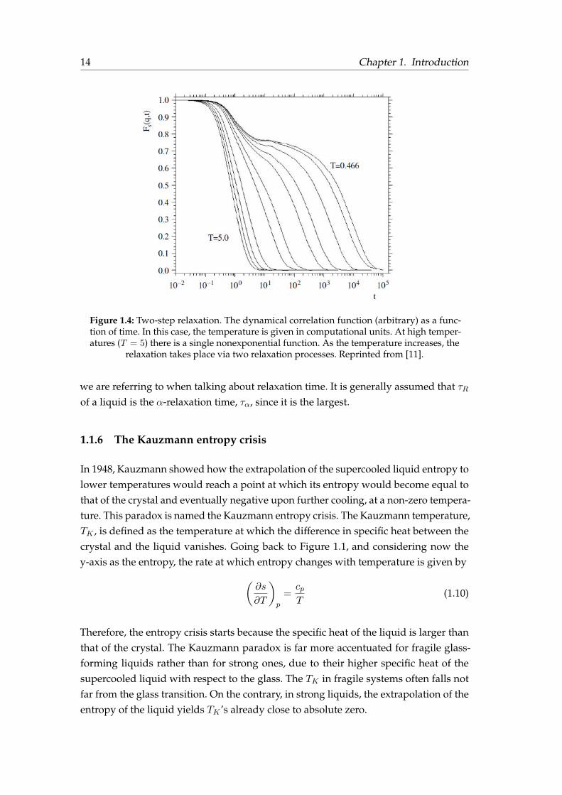
14 Chapter 1. Introduction
Figure 1.4: Two-step relaxation. The dynamical correlation function (arbitrary) as a func-tion of time. In this case, the temperature is given in computational units. At high temper-atures (T = 5) there is a single nonexponential function. As the temperature increases, the
relaxation takes place via two relaxation processes. Reprinted from [11].
we are referring to when talking about relaxation time. It is generally assumed that τRof a liquid is the α-relaxation time, τα, since it is the largest.
1.1.6 The Kauzmann entropy crisis
In 1948, Kauzmann showed how the extrapolation of the supercooled liquid entropy tolower temperatures would reach a point at which its entropy would become equal tothat of the crystal and eventually negative upon further cooling, at a non-zero tempera-ture. This paradox is named the Kauzmann entropy crisis. The Kauzmann temperature,TK , is defined as the temperature at which the difference in specific heat between thecrystal and the liquid vanishes. Going back to Figure 1.1, and considering now they-axis as the entropy, the rate at which entropy changes with temperature is given by(
∂s
∂T
)p
=cpT
(1.10)
Therefore, the entropy crisis starts because the specific heat of the liquid is larger thanthat of the crystal. The Kauzmann paradox is far more accentuated for fragile glass-forming liquids rather than for strong ones, due to their higher specific heat of thesupercooled liquid with respect to the glass. The TK in fragile systems often falls notfar from the glass transition. On the contrary, in strong liquids, the extrapolation of theentropy of the liquid yields TK ’s already close to absolute zero.
1.1. Phenomenology of the glass transition 15
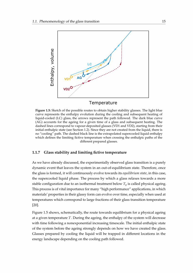
Figure 1.5: Sketch of the possible routes to obtain higher stability glasses. The light bluecurve represents the enthalpy evolution during the cooling and subsequent heating ofliquid-cooled (LC) glass, the arrows represent the path followed. The dark blue curve(AG) accounts for the ageing for a given time of a glass and subsequent heating. Thedashed lines correspond to vapour-deposited glasses (VD1 and VD2), starting from theirinitial enthalpic state (see Section 1.2). Since they are not created from the liquid, there isno “cooling” path. The dashed black line is the extrapolated supercooled liquid enthalpywhich defines the limiting fictive temperature when crossing the enthalpic paths of the
different prepared glasses.
1.1.7 Glass stability and limiting fictive temperature
As we have already discussed, the experimentally observed glass transition is a purelydynamic event that leaves the system in an out-of-equilibrium state. Therefore, oncethe glass is formed, it will continuously evolve towards its equilibrium state, in this case,the supercooled liquid phase. The process by which a glass relaxes towards a morestable configuration due to an isothermal treatment below Tg is called physical ageing.This process is of vital importance for many “high performance” applications, in whichmaterials’ properties in their glassy form can evolve over time, especially when used attemperatures which correspond to large fractions of their glass transition temperature[20].
Figure 1.5 shows, schematically, the route towards equilibrium for a physical ageingat a given temperature T . During the ageing, the enthalpy of the system will decreasewith time following a nonexponential increasing timescale. The initial enthalpic stateof the system before the ageing strongly depends on how we have created the glass.Glasses prepared by cooling the liquid will be trapped in different locations in theenergy landscape depending on the cooling path followed.

16 Chapter 1. Introduction
For instance, let’s consider the three cooling routes shown in Figure 1.1; in a firstand fast cooling (yellow line) the system falls out of the equilibrium at Tg,1. On theother hand, by using slower cooling rates (orange and blue lines), the system will havemore time to equilibrate at a given temperature and will fall out of equilibrium atlower temperatures, Tg,2 and Tg,3, respectively. Therefore, the lower the cooling rate,the lower the glass transition. However, the sharp increase in the relaxation times ofthe supercooled liquids—especially on fragile liquids—will confine the measured Tg
in a narrow range of temperatures, e.g. the Tg changes between 3-5 K for an order ofmagnitude change in the cooling rate [18]. This fact precludes the formation of highlystable glasses—and crystallisation—within human timescales by cooling or ageingprocesses.
The fictive temperature, Tf , is a useful parameter to describe the progress of the glassto lower energy states. This temperature is defined as the temperature at which aproperty of the glass (enthalpy, volume) is equal to that of the supercooled liquid. Attemperatures above the glass transition, the Tf is equal to the physical temperature, aswe are in equilibrium. As the system is cooled, the fictive temperature starts departingfrom equilibrium being Tf > T . At lower temperatures, the system will be completelyarrested reaching a final value of Tf well above the physical temperature. This value iscalled the limiting fictive temperature (T ′f ) [21]. In the cooling scheme shown in Figure1.1, the T ′f coincides typically with the glass transition, obtained from the crossoverbetween the glass enthalpy and the liquid enthalpy. On the other hand, Figure 1.5represents the enthalpy path followed during a heating scan for glasses prepared usingdifferent routes together with the limiting fictive temperature of each one of them. Forinstance, the aged glass prepared at the same cooling rate as the liquid cooled (LC)glass (light-blue curve at Figure 1.5) but physically aged at a temperature Ta will havea lower value of T ′f . The fictive temperature of the glass depends on its thermal historyand the physical temperature of the system as sketched in Figure 1.5. The vapour-deposited glasses sketched in this same figure will be discussed in Section 1.2.
1.1.8 Measuring the glass transition temperature: the heat capacity
The glass transition temperature can be studied using a wide variety of techniques[22] by measuring properties such as the thermal expansion coefficient, the density,the viscosity or the heat capacity. The latter is probably one of the most broadly usedmagnitudes to measure the Tg. The heat capacity measures the amount of heat neededto raise the system’s temperature by one Kelvin. The heat refers to the amount ofenergy transferred into a system other than work and matter. The heat capacity, as anextensive property, depends on the size of the system. The magnitude usually used isthe specific heat capacity or, simply, the specific heat, which is the heat capacity per unitmass. The specific heat depends on the number of degrees of freedom available in a

1.1. Phenomenology of the glass transition 17
Figure 1.6: Schematic representation of the specific heat during a slow cooling (upperdashed line) and a faster heating scan (continuous upper line). The lower curves repre-sent the corresponding enthalpy during the same cooling and heating procedure. Thedashed curve corresponds to the SCL extrapolation line in the enthalpy representation.
The different relevant temperatures are indicated in the sketch.
system. Whereas a gas has translational, rotational and vibrational degrees of freedom,a solid typically only has the vibrational ones, although some other contributions mightbe present in this case—such as magnetic or electronic ones.
Calorimetry is the science or act of measuring the amount of heat exchanged betweena sample during a thermal process, giving access to kinetic and thermodynamic infor-mation of the materials’ state. Information such as heat capacity, enthalpy, entropy orphase transition temperatures can be obtained. As we have already seen, during theglass transition there is a jump in the specific heat due to a sudden reduction in thenumber of available states. Typically, the heat capacity (at constant pressure) measure-ments in glasses are performed during heating temperature ramps. What is usuallymeasured, then, is the devitrification of the glass rather than its formation.
From the heat capacity signature during the devitrification of a glass, several kineticand thermodynamic properties can be readily obtained. Figure 1.6 summarises some ofthe key features from a specific heat scan. The temperature at which the devitrificationtakes place is the onset temperature (Ton) of devitrification. This temperature dependson the kinetics of the experiment. When the heating rate is low, the system has moretime to relax towards the equilibrium at each temperature step so the onset temperaturewill finally be lower than during a faster heating rate scan. When the heating rate andcooling rate are the same, then the glass transition and the onset temperature typicallycoincide (assuming the ageing effects below Tg are negligible, otherwise there would behysteresis effects). That is because the same relaxation path is followed both in cooling
18 Chapter 1. Introduction
and heating. On the other hand, when the heating rate is higher than the cooling, theonset temperature will be shifted to higher temperatures as the system will not havethe same amount of time to relax towards the SCL equilibrium.
Now, for the same heating rate, the onset temperature will scale with the kinetic sta-bility of the glass. In a more stable glass, higher temperatures (or times) are needed todislodge the molecules from their glassy configurations. Besides the jump in specificheat, the heating scan can also be characterised by a peak overshoot, as seen in Figure1.6. The area of this peak is the excess of enthalpy that the system needs to return to theSCL equilibrium state and it is related to the thermodynamic stability of the glass. Theparameter to quantify the thermodynamic stability is the (enthalpic) limiting fictivetemperature. In that case the lower the T ′f , the higher the thermodynamic stability ofthe glass.
In practice, the enthalpic limiting fictive temperature can be obtained from the spe-cific heat data in a heating scan. First, the specific heat is integrated with respect totemperature obtaining the enthalpy (see equation 1.2). Then, the enthalpy line forthe supercooled liquid is extrapolated until it intersects with the integrated enthalpiccurve at T ′f . Figure 1.6 schematically describes the obtaining of the T ′f in a heating scan,equivalently as it is done for a cooling measurement.
1.2 Physical vapour-deposited glasses
Up to now, we have only considered the possibility of creating a glass upon a cool-ing process from the liquid phase. There are, however, other routes to obtain amor-phous solids, such as milling —widely used for pharmaceutical drugs [6]— or physicalvapour deposition. Different techniques such as sputtering deposition, electron beamdeposition or thermal evaporation allow to vapour-depositing glasses. Thermal evap-oration was the technique employed by Hikawa et al. [23] in one of the first workson vapour-deposited glasses. In this work, they prepared VD glasses at substrate tem-peratures corresponding to the 41 % and 69 % of the glass transition of the material,the organic liquid butyronitrile with Tg = 97 K, and compared their thermal responsewith a conventional glass prepared from the liquid. They found that the devitrificationtemperature of the VD glasses was the same for both vapour-deposited glasses and theglass cooled from the liquid. However, they also discovered that the sample depositedat 0.41Tg showed a much higher configurational enthalpy than the sample cooled fromthe liquid while the sample deposited at 0.69Tg lied in-between. They also traced thespontaneous heat evolution during a heating experiment, which is related to the en-thalpy relaxation in an ageing process. The VD samples were unstable and releasedlarge amounts of enthalpy compared to the liquid cooled sample, even well below theTg. They concluded that the molecules deposited on the cold substrate were arrested as

1.2. Physical vapour-deposited glasses 19
they arrived, so the glass got trapped in an entirely different and less stable configura-tion than the LC sample. Later on, similar results were obtained in other systems, suchas 1-pentacene, where the authors concluded, and quoting: “This [higher configurationenthalpy and entropy] indicates that the VQ [vapour-quenched] glass possesses much locally-strained and disordered structure compared with the LQ [liquid-quenched] glass”[24]. Theidea of vapour-deposited glasses (at low temperatures) being less stable than the onescooled from the liquid was extended as a general behaviour to all simple glass-formingmolecules and all deposition temperatures.
In stark contrast to that view, in 2007, physical vapour deposition settled in as an al-ternative way to effectively prepare glasses with significantly enhanced propertiescompared to the liquid cooled ones. Swallen et al. [10] reported how the kinetic re-strictions of the drastic slowdown suffered when cooling a liquid could be bypassedby vapour-depositing the material at the optimal conditions achieving, thus, glasseswhich were much deeper in the potential energy landscape. They used differentialscanning calorimetry to examine the kinetics and thermodynamics of PVD glasses ofthe molecular organic glass-formers 1,3-bis-(1-naphthyl)-5-(2-naphthyl)benzene (TNB)and indomethacin (IMC). When the substrate temperature during the deposition (Tdep)was held at ∼0.85Tg and using low growth rates of 5 nm s−1, glasses with surprisinglylow limiting fictive temperatures (high thermodynamic stability) and high devitrifica-tion onsets (high kinetic stability) were achieved. In Figure 1.5, the enthalpy of vapour-deposited glass versus temperature is sketched for a heating scan together with theenthalpy paths for LC glasses.
As an example, Figure 1.7 shows the calorimetric trace of the devitrification for threedifferently prepared glasses of an organic molecule—TPD— measured by differentialscanning calorimetry. The glass exhibiting the lowest onset for the glass transition andthe smallest overshoot is the glass prepared from the liquid by cooling it at 10 K min−1.On the other hand, the two glasses prepared from the vapour phase at depositiontemperatures of 0.86Tg and 0.90Tg and growth rates of 0.2 nm s−1, exhibit much higheronset temperatures and overshoot, indicating a substantial increase of the kinetic andthermodynamic stabilities.
1.2.1 Stable glass formation mechanism
The mechanism initially proposed by Swallen et al. [10] for the formation of thesestable glasses is based on the higher molecular mobility at the surface compared tothe bulk. The existence of enhanced surface dynamics—in the form of a highly-mobilelayer—has been proven in many systems, from polymers [25] to these same molecularglass-formers systems [26, 27]. For instance, Zhu et al. [27] found that the surface self-diffusion can be up to 106 times greater than the self-diffusion in the bulk.

20 Chapter 1. Introduction
Figure 1.7: Calorimetric trace of the devitrification of three differently prepared glassesof TPD (Tg = 333 K), an organic semiconductor hole transport molecule. CG stands forconventional glass, which is the glass prepared from the liquid. Tdep stands for depositiontemperature of the vapour-deposited glasses at the indicated growth rate. The dashed
lines indicate the determination of the onset temperatures.
When the vapour-deposited molecules arrive at the substrate—at a given T belowTg—they get into this high-mobility surface layer. This mobility allows them to sampletheir best configurations in their potential energy landscape according to the tempera-ture of the substrate during the deposition. If the deposition rate is low enough, thesemolecules can find a favourable configuration before being buried into the bulk bythe subsequent incoming molecules. If the deposition rate is too fast, the moleculesget trapped into the slow dynamics of the bulk before having time to explore a signifi-cant fraction of the configurational space and, therefore, a less stable glass is produced.Typically, when the deposition rate is below 0.5 nm s−1, the stability is no longer im-proved since molecules have “time enough” for the configurational sampling, as seenby different molecular glass-formers [28–30].
The other factor controlling the formation of these glasses is the substrate temperature.Close to Tg, the mobility is high enough so the molecules can find the equilibriumat the corresponding temperature. When the temperature is lowered, the mobilityis reduced but also the configurational phase space. Therefore, the stability will in-crease as the substrate temperature is decreased until the molecules can no longerequilibrate: the mobility will be too low and the equilibration times will exceed thelaboratory timescale. Experimentally, this temperature is found to be ∼0.85Tg for mostvapour-deposited glass-formers, as an indication of a universal behaviour. The glassesdeposited below this temperature will be less stable; the molecules will get trapped asthey arrive at the surface, being able to explore fewer and fewer fractions of the phasespace as temperature decreases.

1.2. Physical vapour-deposited glasses 21
Very recently, Ngai et al. [31] have linked the stable glass formation with the β-relaxation(particularly a subtype of β-relaxation called Johari-Goldstein relaxation). They ratio-nalise it in terms of a secondary glass transition, Tg,β , which they define as the temper-ature at which the β-relaxation time is equal to 1000 s—equivalently yo the standardTg and the α-relaxation1. They found this temperature to be a good indicator of theenhancement of the surface diffusion and, therefore, the capability to form a stableglass. This is still a hot topic since recent data seem to suggest that stable glasses canalso be formed even in molecular systems with very low-surface mobilities [32].
1.2.2 Highly stable glass properties
Originally, in reference [10] from 2007, higher thermal and kinetic stability were re-ported for glasses of IMC and TNB when deposited at 0.85Tg. Since then, highly stableglasses of many other systems (mostly organic) have been produced and their differ-ent properties measured using a broad variety of techniques. Here we list the mostoutstanding characteristics that vapour-deposited glasses exhibit, which have beenmeasured for various materials:
• Higher kinetic stability and lower enthalpies have been seen by differential scanningcalorimetry [28, 33, 34], fast-scanning nanocalorimetry [29, 34], alternating currentnanocalorimetry [35, 36], dielectric relaxation spectroscopy [37, 38], ellipsometry[39, 40], second ion mass spectrometry (SIMS) [41, 42] or inert gas permeation[43] among other techniques. Related to the kinetic stability, highly stable glassesrequire up to 105 times the structural relaxation time of the supercooled liquid tofully transform [41].
• Higher densities: glasses prepared at 0.85Tg can be up to 1.5 % denser than theconventional glass, density variations scale with stability [39, 40, 44, 45]. Thisvariation as a function of Tdep have been reported using mainly ellipsometry, butalso other light interference techniques [46] and X-ray reflectivity measurements[10].
• Enhanced mechanical properties, such as higher mechanical moduli and higher lon-gitudinal sound velocities can also be achieved by properly setting the depositionconditions [39, 47, 48].
• Lower heat capacities, lower expansion coefficient and increased resistance to wateruptake have also been reported for different systems [36, 44, 49].
1We have defined before this time to be 100 s. Since it is a convention, there is no exact definition andsome authors prefer to use 1000 s instead. Anyhow, the accepted range lie between these two values.

22 Chapter 1. Introduction
• Suppression of β-relaxation, it has only been reported on toluene, n-propanol and2-picoline using dielectric relaxation spectroscopy[50]. More recently, it has beenalso shown for the pharmaceutical drug etoricoxib[51].
• Different anisotropic packing that depends on the ratio Tdep/Tg at which the glassis deposited. The degree of molecular orientation and its direction (horizontal orvertical) strongly depends also on the molecular shape. Techniques such as X-raydiffraction [52], ellipsometry using birefringence modelling [44, 45] or dichroismmeasurements [45] have been used to quantify the anisotropy of these glasses.
• Heterogeneous transformation mechanism, which is maybe one of the most excep-tional features of vapour-deposited glasses. While conventional glasses trans-form via a homogenous process, taking place at the whole volume, in VD stableglasses the transformation takes place via a surface-initiated growth front thatpropagates into the bulk. This mechanism has been directly and indirectly ob-served or inferred using several techniques [34, 40–42, 53, 54].
• Suppression of the two-level systems, a feature that was considered to be universalamong all glasses at very low temperatures but that has not been observed inindomethacin ultrastable glasses [55].
Most of the systems that have been reported to form ultrastable glasses are organicmolecules: from simple aromatic hydrocarbons (toluene [29, 30, 35, 43, 46, 53], ethyl-benzene [29, 30, 35, 43, 46, 56], propylbenzene [46] or isopropylbenzene [46] amongothers), pharmaceutical drugs (indomethacin [10, 34], celecoxib [33] and others [57]),general well-known molecular glass-formers (TNB [44], cis/trans-decalin mixtures [58],o-terphenyl [59], tetrachloromethane [60]) to organic semiconductor molecules (TPD,α-NPD or DSA-Ph [45]). More recently some studies on ultrastable metallic glasses[61] and polymers can also be found [62].
Ultrastable glasses have also been produced by computer simulations. In 2010, Léonardand Harrowell [63] used a minimalist model of cooperative dynamics, the facilitatedkinetic Ising model, to reproduce the ultrastable glasses produced by PVD. Using thissimple spin model, they could produce ultrastable glass films that exhibit a front-liketransformation to the supercooled liquid, just as seen experimentally. The melting of ul-trastable glasses using this dynamic facilitation point of view have also been addressedby Gutiérrez and Garrahan [64], who specifically addressed the competition betweenthe bulk and surface transformation mechanisms. Other different approaches to mimicultrastable glasses have also been proposed in molecular dynamics simulations, suchas vapour-depositing Lennard-Jones particles one by one [65], random pinning [66]and particle swapping [67], overcoming in different ways the difficulty of producingin silico VD stable glasses because of the large computational times involved.
1.2. Physical vapour-deposited glasses 23
Vapour-deposited ultrastable glasses have opened a new route to gain access to glasseswith properties equivalent to liquid cooled glasses aged for millions of years [10]. Theyare good candidates to explore the possibility of experimentally determining how theKauzmann entropy crisis can be avoided [28].
The role of fragility in the ability to form highly stable glasses has also been consid-erably discussed. A common feature of the most stable glasses is their fragile nature,and some authors have attempted to establish a straight correlation between these twocharacteristics [61, 68]. This interpretation contrasts with recent results with two lessfragile organic glass-formers (methyl-m-toluate and ethylcyclohexane), which can alsobe prepared in a stable form [38, 69]. The anisotropic packing, which is also a commonfeature in many organic PVD glasses, leads to the discussion of the role that the asym-metry in the molecular structure has in the formation of ultrastable glasses. However,recently Chua et al. [60] have been able to produce stable glasses of tetrachloromethane,which has a nearly spherical structure. Therefore, they ruled out the anisotropy as aprerequisite for the ultrastable glass formation.
As we have seen, there is still an ongoing debate on the mechanisms and characteris-tics behind the vapour-deposited glasses that, at the same time, can provide furtherinsights into the glass transition science. This work is committed to contribute to theunderstanding of the striking properties of these glasses and their possible applicationsin a specific area: the organic light-emitting diodes.


Chapter 2
Experimental methods
In this chapter, we describe the basic methodology followed in this study, coveringfrom the samples’ preparation to their characterisation. This work is based on vapour-deposited organic glasses. Hence, the experimental setup and the materials used inthis work are firstly described. Secondly, the charaterisation techniques are presented.The deposited organic samples have been characterised in situ using membrane-basedmicrofabricated sensors that have been developed at GNaM’s group. Quasi-adiabaticfast-scanning nanocalorimetry and 3ω–Völklein technique working principles are ad-dressed together with a brief description of the well-established 3ω method.
2.1 Experimental setup for physical vapour deposition
Physical vapour deposition is a process where a material, either liquid or solid, is va-porised and transported through a vacuum or low-pressure environment in its basicunits—atoms or molecules—to a substrate, where it condensates. PVD processes aretypically used to prepare thin films with thicknesses than can range from a few atomsto thousands of nanometers. There exist several PVD techniques that are used to pre-pare films of different natures, from various single elements such gold, zinc, aluminiumor silicon (both in crystalline or amorphous forms), alloys such as indium tin oxideor organic molecules such as has been done in this work. These thin films are laterused for several technological and research purposes such as single and multi-layeredcoatings, optical films, decorative coatings, corrosion-resistance films, electrically insu-lating layers in microfabrication processes, active layers in organic electronic devicesamong many others [70]. Among the different methods for PVD processing, the mainones are sputter deposition, arc vapour deposition, ion plating and vacuum deposition.The latter, also called vacuum evaporation, is the method used in this work to evap-orate different organic materials. Vacuum evaporation is a PVD process in which thesource material is thermally evaporated so that the molecules or atoms travel from thevaporisation source to the substrate without any (or few) collisions with the residualgas molecules
26 Chapter 2. Experimental methods
2.1.1 Vacuum evaporation
To achieve a long mean free path of the molecules or atoms, vacuum deposition nor-mally requires vacuum levels better than 10−4 mbar. For example, at 10−6 mbar themean free path of a molecule is already about 5 m and the time needed for the residualspecies to form a monolayer at room temperature is about one second. Therefore, whenthe film contamination is a problem (as it can be in organic films) higher vacuum con-ditions are needed. The high vacuum (HV) levels needed for thermal evaporation areachieved in this work by using a turbomolecular pump attached to a dry scroll pump.Using this configuration ultra-high vacuum (UHV) levels between 10−7 and 10−8 mbarare attained within a few hours. Moreover, we have used the concept of cold trap tofurther reduce the base pressure of the chambers. It consists on a specially designedcopper recipient which can be filled with liquid nitrogen (LN2) from the outside and,therefore, be refrigerated to 77 K (LN2 boiling point at ambient pressure). In the innerpart, the copper surface is maximised using copper disks. Due to the condensationon the cold trap surface of water (and possibly other atmospheric constituents), thepressure of the chamber can decrease up to an order of magnitude, reaching up to 10−8
and 10−9 mbar vacuum levels.
The vapour pressure of a given material strongly depends on the temperature, whichis, therefore, a crucial parameter to set a given evaporation rate. It is generally assumedthat the minimal value of vapour pressure necessary to achieve a useful depositionrate is around 10−2 mbar [71]. In that sense, materials that exhibit this value of vapourpressure at the solid phase are considered sublimating materials whereas materialsthat achieve this value at their liquid phase are described as evaporating materials.
The vaporisation sources used to create the material flux will depend on the character-istics of the materials at room temperature; essentially whether they are liquid or solid.For instance, the aromatic hydrocarbon toluene used in this work is liquid at room tem-perature, with a vapour pressure—35 mbar—high enough to be directly injected into aUHV chamber. If that is the case, the liquid is loaded in a high vacuum pre-chamber,and the deposition rate is controlled using a high precision valve. On the other hand,the other materials used in this work are solid at room temperature and normallyfound in their powder crystalline form. These materials need to be heated above—ornear—their melting point to achieve the necessary vapour pressures to give usefuldeposition rates. To do so, we have used effusion cells that allow an accurate control ofthe temperature and, therefore, of the vapour pressure and the deposition rate of theheated materials. Those evaporators consist basically of a crucible (metallic or quartz)where the materials are loaded and subsequently heated radiatively throughout via ahot filament, achieving highly uniform temperature profiles across the cell.
Vacuum chambers can be equipped with multiple accessories that are needed either
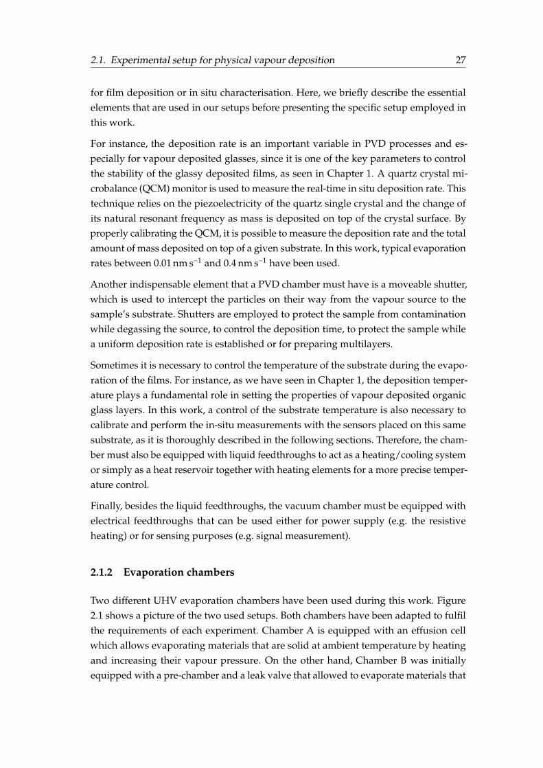
2.1. Experimental setup for physical vapour deposition 27
for film deposition or in situ characterisation. Here, we briefly describe the essentialelements that are used in our setups before presenting the specific setup employed inthis work.
For instance, the deposition rate is an important variable in PVD processes and es-pecially for vapour deposited glasses, since it is one of the key parameters to controlthe stability of the glassy deposited films, as seen in Chapter 1. A quartz crystal mi-crobalance (QCM) monitor is used to measure the real-time in situ deposition rate. Thistechnique relies on the piezoelectricity of the quartz single crystal and the change ofits natural resonant frequency as mass is deposited on top of the crystal surface. Byproperly calibrating the QCM, it is possible to measure the deposition rate and the totalamount of mass deposited on top of a given substrate. In this work, typical evaporationrates between 0.01 nm s−1 and 0.4 nm s−1 have been used.
Another indispensable element that a PVD chamber must have is a moveable shutter,which is used to intercept the particles on their way from the vapour source to thesample’s substrate. Shutters are employed to protect the sample from contaminationwhile degassing the source, to control the deposition time, to protect the sample whilea uniform deposition rate is established or for preparing multilayers.
Sometimes it is necessary to control the temperature of the substrate during the evapo-ration of the films. For instance, as we have seen in Chapter 1, the deposition temper-ature plays a fundamental role in setting the properties of vapour deposited organicglass layers. In this work, a control of the substrate temperature is also necessary tocalibrate and perform the in-situ measurements with the sensors placed on this samesubstrate, as it is thoroughly described in the following sections. Therefore, the cham-ber must also be equipped with liquid feedthroughs to act as a heating/cooling systemor simply as a heat reservoir together with heating elements for a more precise temper-ature control.
Finally, besides the liquid feedthroughs, the vacuum chamber must be equipped withelectrical feedthroughs that can be used either for power supply (e.g. the resistiveheating) or for sensing purposes (e.g. signal measurement).
2.1.2 Evaporation chambers
Two different UHV evaporation chambers have been used during this work. Figure2.1 shows a picture of the two used setups. Both chambers have been adapted to fulfilthe requirements of each experiment. Chamber A is equipped with an effusion cellwhich allows evaporating materials that are solid at ambient temperature by heatingand increasing their vapour pressure. On the other hand, Chamber B was initiallyequipped with a pre-chamber and a leak valve that allowed to evaporate materials that

28 Chapter 2. Experimental methods
are liquid at room temperature. This chamber was later equipped with two effusioncells so multilayers of different materials could be evaporated without breaking thevacuum.
Both UHV chambers have the same elements in common connected to their differentports:
(i) A dry scroll pump Varian SH-110 for generating the primary vacuum, down to6× 10−2 mbar.
(ii) A turbomolecular pump Varian Turbo-V 301 for generating the ultra-high vac-uum, down to ∼2× 10⁻⁸ mbar. A smaller turbomolecular pump Varian Turbo-V81-T is used in the pre-chamber of B.
(iii) A liquid nitrogen (LN2) cold trap is installed on top of both chambers. In chamberB, the cold trap is also used as a cold source and sample holder (later explained).
(iv) A hot cathode Bayard-Alpert gauge to measure the pressure.
(v) A commercial quartz crystal microbalance (QCM) monitor from Sycon Instru-ments. Although the head of the crystal is placed near the sample, a proper cali-bration needs to be performed to determine the ratio between the thickness readby the QCM and the real thickness evaporated at the sample’s position. This isregularly done by measuring control samples using standard profilometry. Themass, when possible, is inferred from the heat capacity measurements.
(vi) A movement feedthrough, either with linear or rotatory motion. At the end of thisfeedthrough a shutter blade is placed to protect the sample from the incomingparticle flux when necessary—i.e. while stabilising the rate, temperature or in-between different sample depositions.
(vii) An electrical feedthrough for sensing and controlling purposes.
2.1.3 Evaporators
As previously described, the requirement for physical vapour deposition is to have thecorresponding material with sufficient vapour pressure.
Chamber B was initially used for materials that are liquid at room temperature, suchas toluene. The liquid to be evaporated is placed in a Pyrex container and put in apre-chamber. The liquid container is coupled with the UHV pre-chamber by openingthe valve. If the liquid vapour pressure is high enough at ambient pressure (as it isfor toluene), the vapour can be introduced to the UHV main chamber through a high-precision leak valve. Otherwise, the pre-chamber can be heated to increase the liquidvapour pressure of the corresponding material. The high-precision leak valve allows a

2.1. Experimental setup for physical vapour deposition 29
Figure 2.1: Photographs of the experimental vacuum chambers (A and B) used in thiswork. The major components are numbered. (i) Primary scroll-pump, (ii) turbomolecularpumps, (iii) cold trap, (iv) pressure sensor, (v) quartz crystal microbalance, (vi) movement
feedthroughs and (vii) electrical feedthroughs.
fine tuning of the amount of vapour entering the main chamber and, therefore, the rateat which the material is arriving at the substrate. Connected to the leak valve, there is acopper pipe with an opening of 4 mm that leads the vapour directly to the sensor. Theend of the pipe is placed 2 cm away from the substrate and centred to the position ofthe sensor device (the sample nanocalorimeter in this case). The distance and the wideopening of the pipe allow part of the material to arrive at the QCM for monitoring therate. Figure 2.2 shows a sketch of part of the setup.
Both chambers are equipped with low-temperature effusion cells for the evaporationof materials that are solid at room temperature. These effusion cells consist basically ofa crucible—stainless steel or quartz—where the raw material is loaded. The crucible isheated by radiation using hot tantalum filaments until the material starts evaporatingor sublimating. A Createc low-temperature effusion cell with a stainless-steel crucibleand an organic material effusion cell (OME) from MBE Komponenten with a quartzcrucible were used in this work. The temperature of both cells was monitored througha K-type thermocouple and controlled with a power source and a PID system. ChamberB, was equipped with both effusion cells in a costume-designed flange to adapt thedirection of each cell flux to the same focal point.

30 Chapter 2. Experimental methods
Figure 2.2: Sketch of the toluene evaporation setup showing the leak-valve and LN2 coldtrap.
Figure 2.3: Photograph of the sample holder used in chamber A with the various elementslabelled.
2.1.4 Sample holders
The sample holder is where the temperature controlled socket with the sensing devicesis located. The sample holder must be refrigerated to act as a controlled bath (heatsink) temperature from which the sample’s socket can be heated, or just cooled. This isachieved in two different ways in the two chambers.
Chamber A has a holder-arm (Figure 2.3) consisting of a liquid feedthrough in whicha copper block is attached and welded to an extreme for a good thermal link. Thecopper block serves as a holder for the sample’s socket while the liquid feedthroughprovides the cooling to the system. Depending on the minimum temperature desired,a refrigerant liquid or liquid nitrogen can be circulated through this piece. In chamberB, the LN2 cold trap is also acting as a heat sink. At the bottom of the trap (as sketchedin Figure 2.2) a copper cover can be attached with screws and, therefore, be at the same
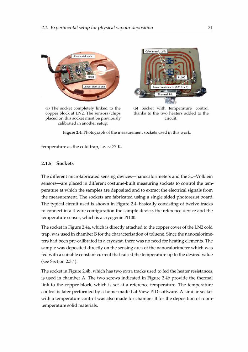
2.1. Experimental setup for physical vapour deposition 31
(a) The socket completely linked to thecopper block at LN2. The sensors/chipsplaced on this socket must be previously
calibrated in another setup.
(b) Socket with temperature controlthanks to the two heaters added to the
circuit.
Figure 2.4: Photograph of the measurement sockets used in this work.
temperature as the cold trap, i.e. ∼ 77 K.
2.1.5 Sockets
The different microfabricated sensing devices—nanocalorimeters and the 3ω–Völkleinsensors—are placed in different costume-built measuring sockets to control the tem-perature at which the samples are deposited and to extract the electrical signals fromthe measurement. The sockets are fabricated using a single sided photoresist board.The typical circuit used is shown in Figure 2.4, basically consisting of twelve tracksto connect in a 4-wire configuration the sample device, the reference device and thetemperature sensor, which is a cryogenic Pt100.
The socket in Figure 2.4a, which is directly attached to the copper cover of the LN2 coldtrap, was used in chamber B for the characterisation of toluene. Since the nanocalorime-ters had been pre-calibrated in a cryostat, there was no need for heating elements. Thesample was deposited directly on the sensing area of the nanocalorimeter which wasfed with a suitable constant current that raised the temperature up to the desired value(see Section 2.3.4).
The socket in Figure 2.4b, which has two extra tracks used to fed the heater resistances,is used in chamber A. The two screws indicated in Figure 2.4b provide the thermallink to the copper block, which is set at a reference temperature. The temperaturecontrol is later performed by a home-made LabView PID software. A similar socketwith a temperature control was also made for chamber B for the deposition of room-temperature solid materials.

32 Chapter 2. Experimental methods
2.1.6 Materials
Five different materials have been used in this work for thin film deposition and sub-sequent measurement of their thermal properties. The organic solvent toluene wasfirst used as a model glass-former. Since it is liquid at room temperature and it has ahigh vapour pressure (38 mbar) its vapour can be directly injected into the UHV cham-ber with the previously described setup. Anhydrous toluene (purity 99.8 %) dried overmolecular sieves and packaged under an argon atmosphere was purchased from CymitQuimica and placed in a Pyrex container which was afterwards connected to a highvacuum pre-chamber. Extra purification of the source material was achieved by apply-ing several sequences of freeze–pump–thaw cycles [29]. Figure 2.5a shows the chemicalstructure for toluene.
Most of the experiments have been performed with the two organic semiconductormolecules TPD (N,N’-Diphenyl-N,N’-di(m-tolyl)benzidine) and α-NPD (N,N’-Di-1-naphthyl-N,N’-diphenylbenzidine) which are both hole transport materials used inorganic electronics. Two other organic semiconductor glass-formers have also been em-ployed in this work: the hole transport material TCTA (4,4’,4”-Tri-9-) and the electrontransport material TPBi (2,2’,2"-(1,3,5-benzinetriyl)-tris(1-phenyl-1-H-benzimidazole).All these materials were purchased in their crystalline powder phase (sublimated grade>99.8 %) from TCI Chemicals and used as received. The melting point of all these ma-terials lies between 448 K and 573 K (see table 2.1). Therefore, it is necessary to use aneffusion cell to get high enough temperatures and reach the desired deposition rates atthe substrate position. Figure 2.5 shows the chemical structure of the molecules.
All five materials exhibit quite distinguishable glass transition temperatures, as listedin table 2.1. Toluene, as it has a unique nature compared to the other materials, hasits glass transition at 117 K and a more simplified molecular structure. For TPD andα-NPD the calorimetric glass transition was measured with a standard differentialscanning calorimetry (DSC7, Perkin Elmer) by cooling the glass at 10 K min−1 andmeasured during a heating scan at the same rate. For the latter two, the glass transitionwas directly taken from the literature.
Mass determination in nanocalorimetry measurements
With quasi-adiabatic fast-scanning nanocalorimetry, one obtains the heat capacity ofthe sample deposited on top of the sensor (further details are provided in Section 2.3).The mass of the sensed sample can be directly obtained from the quotient between theheat capacity and the specific heat, provided that the latter is known. In this work, foreach calorimetric scan, the mass has been obtained by dividing the heat capacity of thesample in the temperature range after the glass transition—that is, in the supercooled

2.1. Experimental setup for physical vapour deposition 33
(a) Toluene
(b) TPD (c) α-NPD
(d) TPBi (e) TCTA
Figure 2.5: Chemical structure of the different molecules used in this work.
Material Tg [K] Tm [K] ρ [g cm−3]
Toluene 117 [72] 178 1.028 [46]TPD 333† 448-450 1.08 [73]α-NPD 368† 552-556 1.22 [73]
TPBi 395‡ 546-550 1.25‡
TCTA 424‡ 571-573 1.15‡
Table 2.1: Basic materials properties for this work: melting and glass transition temperatureand density (at room temperature for the organic semiconductors and at 120 K for toluene).† Glass transition temperatures obtained from conventional DSC by cooling and heatingthe sample at 10 K min−1. ‡ Data taken from the internal database of the Dresden IntegratedCenter for Applied Physics and Photonic Materials (IAPP). All the melting temperatures
are the ones reported by the supplier.
liquid region—by the specific heat at this same temperature range. In doing so, weare always assuming that the supercooled liquid is always the same, regardless the

34 Chapter 2. Experimental methods
original glassy state.
For toluene, the specific heat is well reported by Yamamuro et al. [72] for the whole liq-uid and supercooled liquid range. On the other hand, the specific heats of the differentorganic semiconductors used in this work are barely reported in the literature, and norecords of their value were found. In these cases, a previous calibration was performedto obtain the specific heat value of the evaporated samples. First, a sample of ∼100 nmwas deposited simultaneously on the nanocalorimeter and a silicon wafer, close to eachother during the evaporation. The calorimetric scan was performed as usual to get theheat capacity. The thickness of the sample was measured using standard profilometry.In this way, the mass deposited on the calorimeter could also be inferred by knowingthe sensing area of the chip and the density of the material—more easily found in theliterature. The densities are also reported in table 2.1. The specific heat obtained fromthe mass normalisation of the performed heat capacity scan was later used to get themass of the subsequent samples as described in the previous passage.
The accuracy of this procedure to get the specific heat for the organic semiconductors islow, estimated to be∼10 %, due to the multiple sources of uncertainties in determiningsuch small masses. Errors might come from the thickness determination, density val-ues found in the literature or the sensing area determination. However, the precisionand reproducibility of the technique allow us to measure small differences betweendifferent samples through the calorimetric scans regardless of the possible lack of ac-curacy, which will affect all the samples equally without affecting the conclusions ofthe attained results. Probably, the larger consequences due to this lack of accuracyare found in the determination of the limiting fictive temperature. The main problemcomes from the large extrapolation that must be done of the liquid’s enthalpy curve,more precisely, from the specific heat integration over temperature. This fact is furtherand more extensively addressed in Chapter 3.
2.2 Thermal characterisation techniques
We have used two main characterisation techniques: quasi-adiabatic fast-scanning na-nocalorimetry to obtain the heat capacity (Cp) and the 3ω–Völklein technique to mea-sure the thermal conductance (G). We first provide some brief notes on the equationsgoverning the heat transfer in a simplified system. In this way we pretend to illustratethe characteristics of our thermal sensors and how it is possible to obtain either Cp orG data.

2.2. Thermal characterisation techniques 35
Figure 2.6: Sketch of a calorimeter system as a thermal circuit consisting of a thermal massC at a temperature T and connected to a heat bath at T0 through a thermal conductance G.
Q represents the injected power.
From the energy conservation principle and Fourier’s law for heat conduction, it is pos-sible to derivate the parabolic differential equation that describes the heat distribution—and temperature T—inside a given spatial region over time [74]:
ρc∂T
∂t−∇ · (k∇T ) = q (2.1)
where ρ is the density of the medium, c the specific heat, k the thermal conductivityand q the heat flux per unit volume. We need to solve this equation for our thermalsensors. We can simplify our system/sensor as a solid with a heat capacityC connectedto a heat bath at T0 by a thermal conductance G, as sketched in Figure 2.6. Integratingequation 2.1 over the volume V of a solid and using the Gauss’ theorem in the secondleft-hand term (assuming the surface of the volume to be A and the gradient pointingtowards this surface), it leads to:
C∂T
∂t+ k∇T = Q (2.2)
where C is the heat capacity (C = ρV c), and Q = qV the total power exchanged withthe system. We can simplify even further equation 2.2 by linearizing the gradient as∇T = ∆T/L, obtaining:
C∂T
∂t+G∆T = Q (2.3)
where we have defined the thermal conductance from the solid to the thermal bath asG = kA/L.
Equation 2.3 reflects the conservation of energy of the system. The heat generatedinside the solid is spent either in the dynamic heating (first term) or in heat conductionthrough the thermal link (second term). When there is no heat generation but an initialtemperature mismatch between the two bodies (calorimeter and heat bath), equation2.3 has the trivial solution
∆T = ∆T0 exp (−t/τ) (2.4)

36 Chapter 2. Experimental methods
where we have defined τ = C/G as the characteristic time of the system. The evalua-tion of this parameter is of vital importance for any thermal sensor and for the thermalproperties that need to be measured. Let’s study two cases: (i) for t >> τ the systemwill have time to relax towards the equilibrium—i.e. the initial temperature gradientgoes to zero—and therefore, reaches the steady state. If all the power is spent on heatdissipation, it is possible to directly extract the thermal conductance between the sys-tem and the heat bath. (ii) On the contrary, for t << τ , the system will have no timeto dissipate all the input power, which will be used to heat the system dynamically,increasing its temperature. In this case, the system behaves in an adiabatic mode (or inthe so-called quasi-adiabatic mode if the heat losses are small), making it possible toextract the heat capacity of our system directly. Both strategies, (i) and (ii), will be thebasis for the thermal characterisation techniques used in this work.
The demand in science and, specifically, in nanoscience, for measuring smaller andsmaller systems, has forced the characterisation techniques to equally evolve to higherand higher sensitivities by reducing the size of the sensing element. Thanks to theadvances in microfabrication techniques it is possible to fabricate devices with reducedmass and size capable of developing multiple functions. It is in that scenario wherea new family of membrane-based calorimetry techniques have appeared. These tech-niques rely on the use of thin dielectric free-standing membranes (∼150 nm), generallymade of silicon nitride. These membranes serve as a substrate to hold the actuators onone side and transducers required for the calorimetric measurements on the other side,the sample under study. In the following sections, we describe two of these techniques:fast-scanning nanocalorimetry and the 3ω–Völklein technique. The former is used tomeasure the heat capacity while the latter is used to measure the in-plane thermalconductivity.
2.3 Fast-scanning quasi-adiabatic nanocalorimetry
Calorimetry is the science that measures the heat transfer in a body to follow its statevariables, whose changes are associated to physical changes, phase transitions or chem-ical reactions. More particularly, nanocalorimetry is a characterisation technique thatallows measuring the small amounts of energy that are involved in thermal processesof nano-sized systems. A complete calorimetric measurement requires the simultane-ous monitoring of the temperature evolution, the injected power and the heat losses tothe surroundings. The first two quantities can be readily measured by placing a singleplatinum thin film on top of the membrane (∼180 nm), which acts both as a heaterand as a sensor. The fact of having a two-in-one heater and sensor together with theultrathin membrane yields a very low mass for the calorimetric cell (CC). The planargeometry of the membrane provides excellent vertical heat diffusion, ensuring vertical

2.3. Fast-scanning quasi-adiabatic nanocalorimetry 37
temperature homogeneity between the metallic heater and the sample, even for highheating rates (up to 106 K s−1). Moreover, due to the reduced thickness of the mem-brane, the lateral heat diffusion is limited and—in high vacuum conditions—providesan efficient thermal insulation between the sensing area (the calorimetric cell) and thesurroundings. Taking advantage of this fact, we can minimise the heat losses to thesurroundings using fast-heating rates, which are easily achieved due to the low massof the calorimetric cell. The working principle behind quasi-adiabatic fast-scanningnanocalorimetry relies, precisely, on the use of very high heating rates produced by theinjection of short current pulses [75–77].
The use of a calorimeter with a calorimetric cell with low heat capacity permits achiev-ing high sensitivities. By performing differential measurements, it is even possible tomeasure samples with much smaller masses than the calorimetric cell itself. Moreover,using high heating rates also provides several advantages when measuring the heatcapacity. First, it minimises—making it almost negligible—any heat transfer to the sur-roundings, with the cell behaving quasi-adiabatically. Secondly, it reduces the noise ofthe calorimetric signal and, therefore, the heat capacity for smaller samples can be re-solved. Third and last, it also ensures a good temperature profile in the sensor/heatingelement, necessary for accurate measurements of the heat capacity.
2.3.1 Nanocalorimeter description
Figure 2.7 shows a sketch of the nanocalorimeter device used in this work, consistingof a microfabricated silicon chip. A silicon frame holds a 3×6 mm2 silicon nitride free-standing membrane with a thickness of 180 nm. On top of this membrane and at itscentre, a 100 nm thick platinum film in the form of a serpentine circuit is depositedtogether with four contacts for the external connection. These four contacts, two forfeeding with the current and two for sensing the voltage drop, permit the metallicelement to act both as heating and sensing element. With this 4-wire configuration, seeFigure 2.8a, it is possible to measure the amount of power released only in the centralarea—referred as the sensing area—which has a surface of 1.085 mm2.
2.3.2 Principle of operation
The principle of operation of the nanocalorimeters is the Joule effect. The power re-leased to the sensing area is Pin(t) = I(t)V (t). The temperature can be determinedby the resistance of the heating element, R(t) = V (t)/I(t). The resistance dependenceof the platinum strip must be previously calibrated, a procedure that is described inSection 2.5.2.
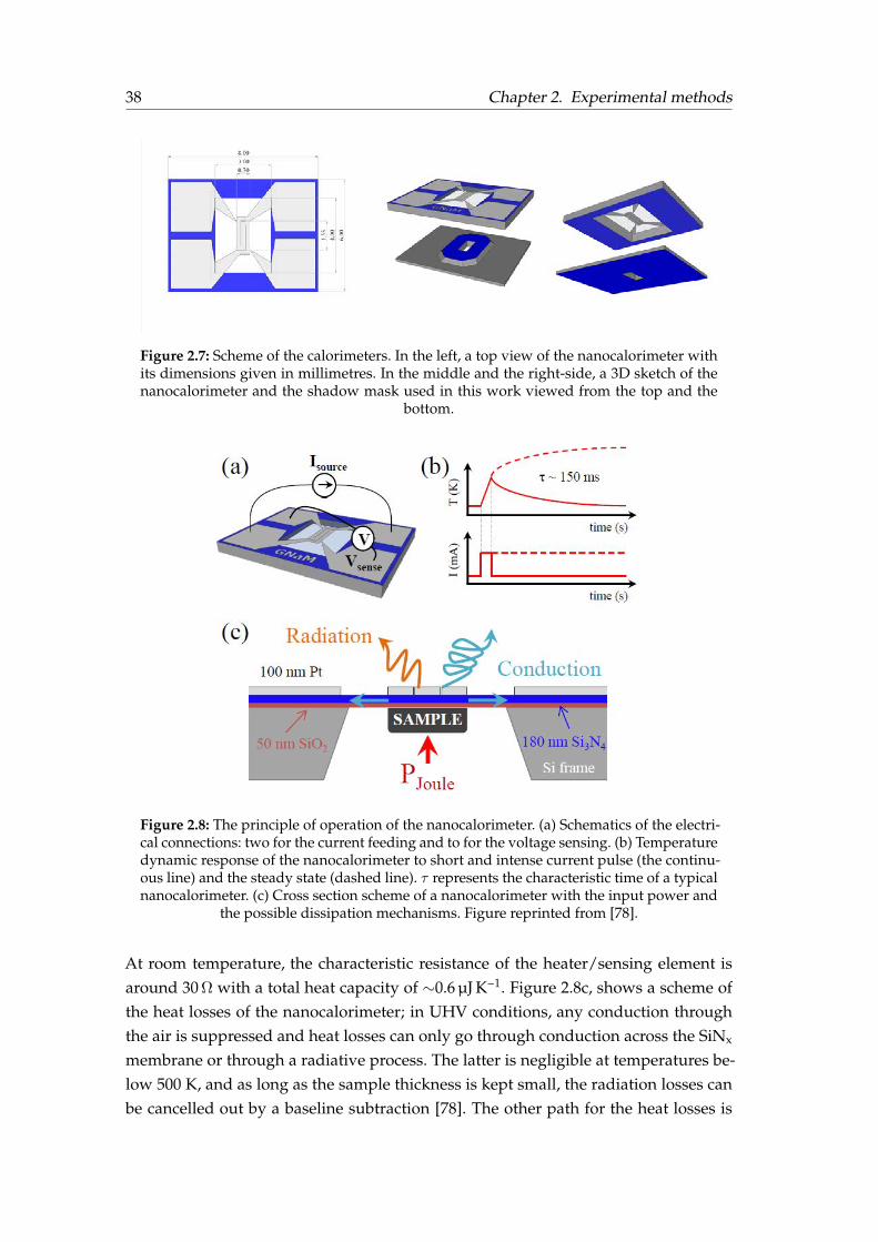
38 Chapter 2. Experimental methods
Figure 2.7: Scheme of the calorimeters. In the left, a top view of the nanocalorimeter withits dimensions given in millimetres. In the middle and the right-side, a 3D sketch of thenanocalorimeter and the shadow mask used in this work viewed from the top and the
bottom.
Figure 2.8: The principle of operation of the nanocalorimeter. (a) Schematics of the electri-cal connections: two for the current feeding and to for the voltage sensing. (b) Temperaturedynamic response of the nanocalorimeter to short and intense current pulse (the continu-ous line) and the steady state (dashed line). τ represents the characteristic time of a typicalnanocalorimeter. (c) Cross section scheme of a nanocalorimeter with the input power and
the possible dissipation mechanisms. Figure reprinted from [78].
At room temperature, the characteristic resistance of the heater/sensing element isaround 30 Ω with a total heat capacity of ∼0.6 µJ K−1. Figure 2.8c, shows a scheme ofthe heat losses of the nanocalorimeter; in UHV conditions, any conduction throughthe air is suppressed and heat losses can only go through conduction across the SiNx
membrane or through a radiative process. The latter is negligible at temperatures be-low 500 K, and as long as the sample thickness is kept small, the radiation losses canbe cancelled out by a baseline subtraction [78]. The other path for the heat losses is
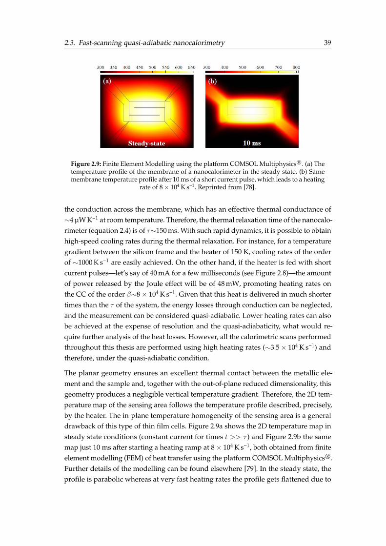
2.3. Fast-scanning quasi-adiabatic nanocalorimetry 39
Figure 2.9: Finite Element Modelling using the platform COMSOL Multiphysics R©. (a) Thetemperature profile of the membrane of a nanocalorimeter in the steady state. (b) Samemembrane temperature profile after 10 ms of a short current pulse, which leads to a heating
rate of 8× 10⁴ K s−1. Reprinted from [78].
the conduction across the membrane, which has an effective thermal conductance of∼4 µW K−1 at room temperature. Therefore, the thermal relaxation time of the nanocalo-rimeter (equation 2.4) is of τ∼150 ms. With such rapid dynamics, it is possible to obtainhigh-speed cooling rates during the thermal relaxation. For instance, for a temperaturegradient between the silicon frame and the heater of 150 K, cooling rates of the orderof ∼1000 K s−1 are easily achieved. On the other hand, if the heater is fed with shortcurrent pulses—let’s say of 40 mA for a few milliseconds (see Figure 2.8)—the amountof power released by the Joule effect will be of 48 mW, promoting heating rates onthe CC of the order β∼8× 10⁴ K s−1. Given that this heat is delivered in much shortertimes than the τ of the system, the energy losses through conduction can be neglected,and the measurement can be considered quasi-adiabatic. Lower heating rates can alsobe achieved at the expense of resolution and the quasi-adiabaticity, what would re-quire further analysis of the heat losses. However, all the calorimetric scans performedthroughout this thesis are performed using high heating rates (∼3.5× 10⁴ K s−1) andtherefore, under the quasi-adiabatic condition.
The planar geometry ensures an excellent thermal contact between the metallic ele-ment and the sample and, together with the out-of-plane reduced dimensionality, thisgeometry produces a negligible vertical temperature gradient. Therefore, the 2D tem-perature map of the sensing area follows the temperature profile described, precisely,by the heater. The in-plane temperature homogeneity of the sensing area is a generaldrawback of this type of thin film cells. Figure 2.9a shows the 2D temperature map insteady state conditions (constant current for times t >> τ ) and Figure 2.9b the samemap just 10 ms after starting a heating ramp at 8× 10⁴ K s−1, both obtained from finiteelement modelling (FEM) of heat transfer using the platform COMSOL Multiphysics R©.Further details of the modelling can be found elsewhere [79]. In the steady state, theprofile is parabolic whereas at very fast heating rates the profile gets flattened due to
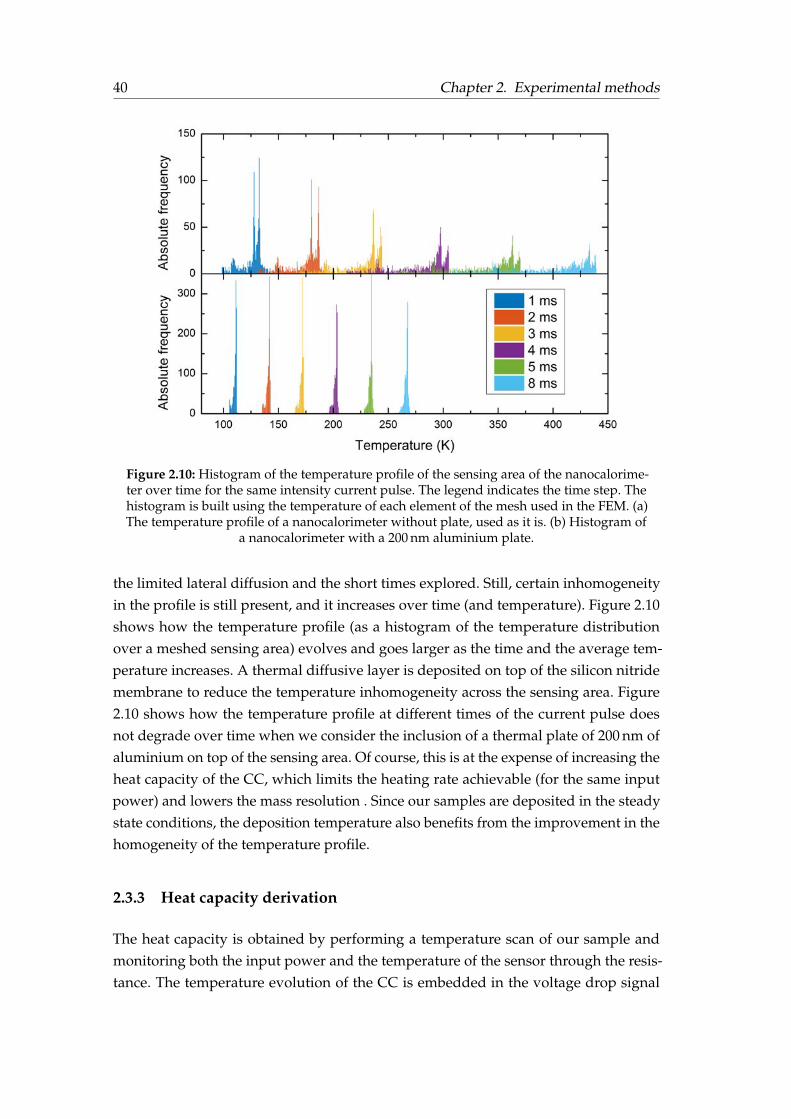
40 Chapter 2. Experimental methods
Figure 2.10: Histogram of the temperature profile of the sensing area of the nanocalorime-ter over time for the same intensity current pulse. The legend indicates the time step. Thehistogram is built using the temperature of each element of the mesh used in the FEM. (a)The temperature profile of a nanocalorimeter without plate, used as it is. (b) Histogram of
a nanocalorimeter with a 200 nm aluminium plate.
the limited lateral diffusion and the short times explored. Still, certain inhomogeneityin the profile is still present, and it increases over time (and temperature). Figure 2.10shows how the temperature profile (as a histogram of the temperature distributionover a meshed sensing area) evolves and goes larger as the time and the average tem-perature increases. A thermal diffusive layer is deposited on top of the silicon nitridemembrane to reduce the temperature inhomogeneity across the sensing area. Figure2.10 shows how the temperature profile at different times of the current pulse doesnot degrade over time when we consider the inclusion of a thermal plate of 200 nm ofaluminium on top of the sensing area. Of course, this is at the expense of increasing theheat capacity of the CC, which limits the heating rate achievable (for the same inputpower) and lowers the mass resolution . Since our samples are deposited in the steadystate conditions, the deposition temperature also benefits from the improvement in thehomogeneity of the temperature profile.
2.3.3 Heat capacity derivation
The heat capacity is obtained by performing a temperature scan of our sample andmonitoring both the input power and the temperature of the sensor through the resis-tance. The temperature evolution of the CC is embedded in the voltage drop signal

2.3. Fast-scanning quasi-adiabatic nanocalorimetry 41
due to the R(T ) dependence of the platinum sensor.
The highest sensitivity and resolution can be obtained when the measurement is per-formed in differential mode. Using a pair of twin calorimeters, that is, with similar heatcapacity and temperature coefficient of resistance (TCR, see Section 2.5.2), the differ-ential voltage between them in a heating temperature scan will be close to zero. Now,if one nanocalorimeter has a sample deposited, the differential voltage between thesample and the reference calorimeters will correspond solely to the calorimetric signalgenerated by the sample itself. This signal, generally small, can be heavily amplifiedusing instrumental amplifiers to accommodate it to the typical ±10 V range of a digitaldata acquisition (DAQ) system. This is the key point of differential nanocalorimetrythat allows obtaining high sensitivities and resolutions.
Under the assumption of adiabatic conditions, the delivered energy is spent into pro-moting the temperature of the system. This temperature increase is proportional to theheat capacity of the system
Cp(T )dT = Pindt (2.5)
We can express the input power, Pin in terms of the measured variables, in that case,the heat capacity reads,
Cp(T ) =V (t)I(t)
β(t)(2.6)
where we have defined the temperature variation with time as the heating rate β(t).It is important to note that all the magnitudes are a function of time. For simplicity,this dependence will not be shown explicitly from now on. Now, if using the differen-tial configuration, the heat capacity of the measured samples will be the differentialcalorimetric signal of both sensors
∆Cp(T (t)) =VSISβS− VRIR
βR=IRVRβR
(VSISβSVRIRβR
− 1
)(2.7)
where subscripts S and R stand for sample and reference, respectively. We can considersome simplification of our analysis before continuing:
(i) In our case, the calorimeters are fed with a constant current pulse. Hence, theintensity is constant throughout time. In that case, since V = IR, voltage andresistance derivative are directly related by dV = d(IR) = IdR.
(ii) Both devices, the sample and the reference, are connected in series to ensure thatthey are fed with the same current. Therefore, we can write IS = IR = I .
(iii) The signal containing the sample’s information is the differential voltage, ∆V ,which can be heavily amplified compared to the single calorimeter signal. We canuse the relation VS = VR + ∆V to include the measured signal.
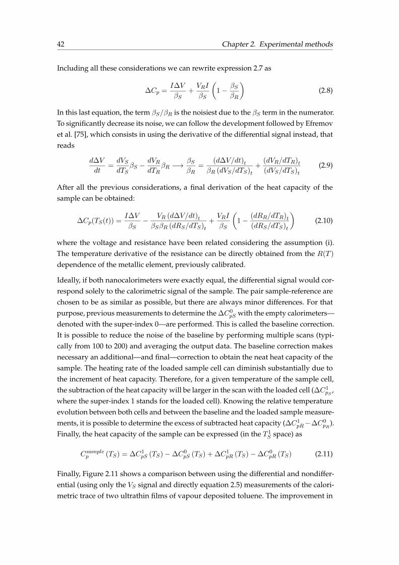
42 Chapter 2. Experimental methods
Including all these considerations we can rewrite expression 2.7 as
∆Cp =I∆V
βS+VRI
βS
(1− βS
βR
)(2.8)
In this last equation, the term βS/βR is the noisiest due to the βS term in the numerator.To significantly decrease its noise, we can follow the development followed by Efremovet al. [75], which consists in using the derivative of the differential signal instead, thatreads
d∆V
dt=dVSdTS
βS −dVRdTR
βR −→βSβR
=(d∆V/dt)t
βR (dVS/dTS)t+
(dVR/dTR)t(dVS/dTS)t
(2.9)
After all the previous considerations, a final derivation of the heat capacity of thesample can be obtained:
∆Cp(TS(t)) =I∆V
βS−
VR (d∆V/dt)tβSβR (dRS/dTS)t
+VRI
βS
(1−
(dRR/dTR)t(dRS/dTS)t
)(2.10)
where the voltage and resistance have been related considering the assumption (i).The temperature derivative of the resistance can be directly obtained from the R(T )
dependence of the metallic element, previously calibrated.
Ideally, if both nanocalorimeters were exactly equal, the differential signal would cor-respond solely to the calorimetric signal of the sample. The pair sample-reference arechosen to be as similar as possible, but there are always minor differences. For thatpurpose, previous measurements to determine the ∆C0
pS with the empty calorimeters—denoted with the super-index 0—are performed. This is called the baseline correction.It is possible to reduce the noise of the baseline by performing multiple scans (typi-cally from 100 to 200) and averaging the output data. The baseline correction makesnecessary an additional—and final—correction to obtain the neat heat capacity of thesample. The heating rate of the loaded sample cell can diminish substantially due tothe increment of heat capacity. Therefore, for a given temperature of the sample cell,the subtraction of the heat capacity will be larger in the scan with the loaded cell (∆C1
pS,
where the super-index 1 stands for the loaded cell). Knowing the relative temperatureevolution between both cells and between the baseline and the loaded sample measure-ments, it is possible to determine the excess of subtracted heat capacity (∆C1
pR−∆C0pR
).Finally, the heat capacity of the sample can be expressed (in the T 1
S space) as
Csamplep (TS) = ∆C1pS (TS)−∆C0
pS (TS) + ∆C1pR (TS)−∆C0
pR (TS) (2.11)
Finally, Figure 2.11 shows a comparison between using the differential and nondiffer-ential (using only the VS signal and directly equation 2.5) measurements of the calori-metric trace of two ultrathin films of vapour deposited toluene. The improvement in
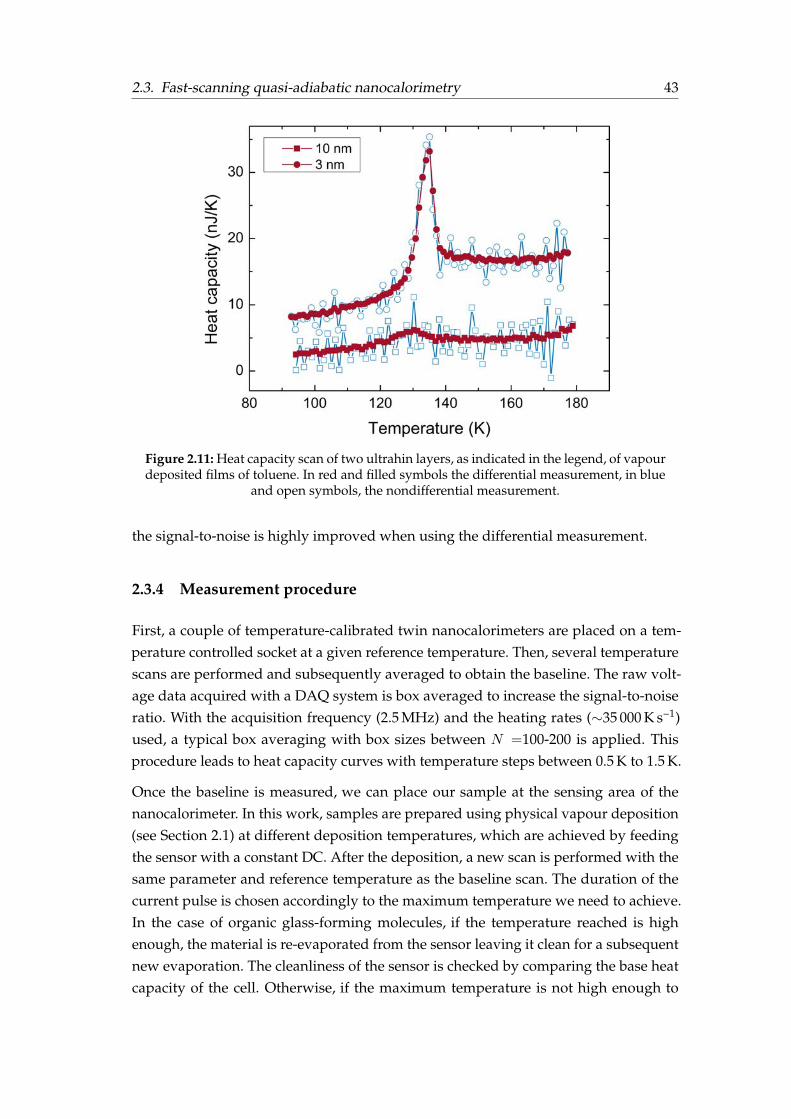
2.3. Fast-scanning quasi-adiabatic nanocalorimetry 43
Figure 2.11: Heat capacity scan of two ultrahin layers, as indicated in the legend, of vapourdeposited films of toluene. In red and filled symbols the differential measurement, in blue
and open symbols, the nondifferential measurement.
the signal-to-noise is highly improved when using the differential measurement.
2.3.4 Measurement procedure
First, a couple of temperature-calibrated twin nanocalorimeters are placed on a tem-perature controlled socket at a given reference temperature. Then, several temperaturescans are performed and subsequently averaged to obtain the baseline. The raw volt-age data acquired with a DAQ system is box averaged to increase the signal-to-noiseratio. With the acquisition frequency (2.5 MHz) and the heating rates (∼35 000 K s−1)used, a typical box averaging with box sizes between N =100-200 is applied. Thisprocedure leads to heat capacity curves with temperature steps between 0.5 K to 1.5 K.
Once the baseline is measured, we can place our sample at the sensing area of thenanocalorimeter. In this work, samples are prepared using physical vapour deposition(see Section 2.1) at different deposition temperatures, which are achieved by feedingthe sensor with a constant DC. After the deposition, a new scan is performed with thesame parameter and reference temperature as the baseline scan. The duration of thecurrent pulse is chosen accordingly to the maximum temperature we need to achieve.In the case of organic glass-forming molecules, if the temperature reached is highenough, the material is re-evaporated from the sensor leaving it clean for a subsequentnew evaporation. The cleanliness of the sensor is checked by comparing the base heatcapacity of the cell. Otherwise, if the maximum temperature is not high enough to

44 Chapter 2. Experimental methods
evaporate the material again, a so-called fast-cooled (FC) glass is created on top ofthe sensing area of the nanocalorimeter. Due to the low mass of the calorimetric celland once the input power is cut, the passive cooling rates achieved are on the orderof 500 K s−1 to 1000 K s−1. These fast rates produce very low stability glasses. Contraryto the VD glass, which needs to be evaporated each time, the creation of the FC glassis reversible and can be measured several times—tenths to hundreds—allowing toaverage all the curves and to obtain much better statistics of the calorimetric trace.For the VD glasses, especially the thinnest (<50 nm), the calorimetric traces shown aretypically the result of averaging the data from 2-10 equally prepared samples (samethickness, same Tdep).
2.4 Thermal conductivity: the 3ω-Völklein method
The 3ω–Völklein is a combination of a widely used method—the 3ω—and the Völkleinmethod for measuring the thermal conductivity of different insulating materials. The3ω method was first described by Cahill in 1990 [80] and was primarily intended formeasuring bulk materials. It consists in depositing a metal strip on top of the sampleunder test and feed it with an alternating-current (AC) at a given frequency ω. Due tothe self-heating of the metallic strip, the voltage through the strip will exhibit a thirdharmonic component. This V3ω can be directly related to the temperature gradientgenerated at the substrate which, in turn, is linked to the thermal conductivity. Thismethod was later adapted for measuring thin film samples in the out-of-plane direction(k⊥) [81, 82]. This latter modification is briefly detailed in Section 2.4.2. However, theVölklein method was introduced in 1997 by Völklein and Starz [83]. They presented amembrane-based sensor that operated in direct-current (DC) mode to measure the in-plane thermal conductance (k‖) of thin films. However, the measurements of thermalconductance were limited to metallic samples and thicknesses lower than 1 µm. Thislimitation was later circumvented by Sikora et al. [84] in 2012, who presented a methodto measure thermal conductivity of very thin suspended membranes based on a mix ofthe 3ω method and the Völklein method, achieving a high sensitivity, up to 10 nW K−1,and a high resolution ∆G/G ' 10−3.
Figures 2.12a and 2.12b show a scheme of the 3ω method for thin films and the 3ω-Völ-klein method for the out and in-plane measurements. The arrows indicate the maindirection of the heat flux for each method, further detailed in the following sections.The light grey represents the metallic element (e.g. platinum) needed for injecting thepower, the dark-grey represents the thin film sample and/or free-standing membranewhereas the black corresponds to the substrate (e.g. silicon).
At GNaM’s, we have developed a modification of the 3ω–Völklein technique that al-lows measuring in situ the thermal conductance of thin films, from either insulating

2.4. Thermal conductivity: the 3ω-Völklein method 45
(a) Geometry for the 3ω to obtain the out-of-planethermal conductivity of the film (dark-grey).
(b) Geometry for the Völklein and 3ω–Völklein to ob-tain the in-plane thermal conductivity of the mem-
brane plus film system (dark-grey).
Figure 2.12: Schematic representation (top and side-view) of the heat flux for the 3ω and the3ω–Völklein geometries. The light-grey describes the metallic elements, the dark grey thefilm under study (or membrane) and the black the substrate or frame. The arrows indicatethe direction of the heat flux, the main direction is described by the arrows’ thickness. Therelevant lengths are also indicated: 2w is the width of the sensor, L the length of the strip,t the thickness of the membrane plus sample and l the width of the membrane for the
3ω–Völklein geometry.
or thermally and electrically conductive material. The high resolution achieved allowsmonitoring the thermal conductance during layer growth by PVD even from the veryfirsts stages (less than one nanometer thick).

46 Chapter 2. Experimental methods
(a) 3D sktech showing thetop and bottom view.
(b) Optical image. (c) Photograph of the sen-sor
Figure 2.13: Different images describing the 3ω–Völklein sensor.
2.4.1 Device description
The thermal sensor developed at GNaM is based—as the nanocalorimeters were—on ametallic sensor built on top of a free-standing SiNx membrane. Two parallel platinumstrips are deposited on top of the membrane, as can be seen from the different imagesin Figure 2.13, each one of the strips prepared to be connected in a 4-wire configuration.For the more standard DC operation (Völklein method), both platinum lines are usedto measure the thermal conductance of the membrane (or membrane plus sample)beneath the two probes exclusively . The measurements performed in this thesis aredone in the AC mode, for which we only use of the central strip, assuming the frametemperature to be the same as the temperature probe were the sensors are placed (seeSection 2.1.5).
The geometry of the sensors was previously optimised [85] using finite element mod-elling with the platform COMSOL Multiphysics R© to ensure the temperature homo-geneity between the voltage probes. The fabricated sensor consists of a membranewith an area of 3 mm× 250 µm and 180 nm thick. The two platinum sensing strips are3 mm× 5 µm and have a thickness of 100 nm. The voltage probes are separated by2 mm. Further details on the sensor optimisation can be found elsewhere [85].
2.4.2 Principle of operation
The principle of operation of this type of sensor is the same as in the nanocalorimeterdevice: the self-heating of the metallic element due to the Joule effect together withits duality as heater and sensor. The main difference here is that we are using ACof a certain angular frequency ω to promote a temperature rise that will generate avoltage component in 3ω due to the self-heating of the metallic strip. This voltage is
2.4. Thermal conductivity: the 3ω-Völklein method 47
used to quantify the amplitude of the temperature oscillations and later extract theconductance of the film/substrate beneath the sensor.
The generation of the V3ω can be derived from the evolution of the dissipated powerto the sensor. First, we feed the sensor with AC with an angular frequency ω = 2πf ,
I = I0 sin (ωt) (2.12)
which produces a dissipated power of
Q = I2R = I20R sin2 (ωt) =I20R
2(1− cos (2ωt)) = Q0 (1− cos (2ωt)) (2.13)
where we have defined the quantity Q0 = I20R/2. Therefore, the dissipated power hastwo components. The first, the DC component, will produce a transient self-heatingthat tends to a constant temperature value for times t >> τ , where τ is the characteristicthermal constant of the system. The second term produces a temperature evolution thatoscillates with time. We can define the temperature steps produced for each componentas
∆TDC ≡Q0
Gand ∆T2ω ≡
Q0
G2ω(2.14)
where we have introduced the apparent conductance G2ω. Due to the permanentlytransient state of the time-dependent term, part of the heat will be expended in dy-namically heating the sensor. Therefore, the G2ω will always be lower than the realconductance. In a more general framework, the temperature oscillation can also be outof phase with respect to the heating wave,
limt→∞
∆T = ∆TDC − |∆T2ω| cos (2ωt+ φ) (2.15)
These temperature oscillations will be translated into resistance oscillations too,
R = R0 +dR
dT∆T = R0 +
dR
dT(∆TDC −∆T2ω cos (2ωt+ φ)) (2.16)
which, in turn, will affect the voltage of the strip through the Ohm’s law,
V = I0
(R0 +
dR
dT∆TDC
)sin (ωt)− I0∆T2ω
dR
dTsin (ωt) cos (2ωt+ φ) (2.17)
The last term can be rewritten using trigonometrical identities, leading to the followingexpression:
V = I0
(R0 +
dR
dT∆TDC
)sin (ωt) + I0
∆T2ω2
dR
dTsin (ωt+ φ)
−I0∆T2ω
2
dR
dTsin (3ωt+ φ)
(2.18)
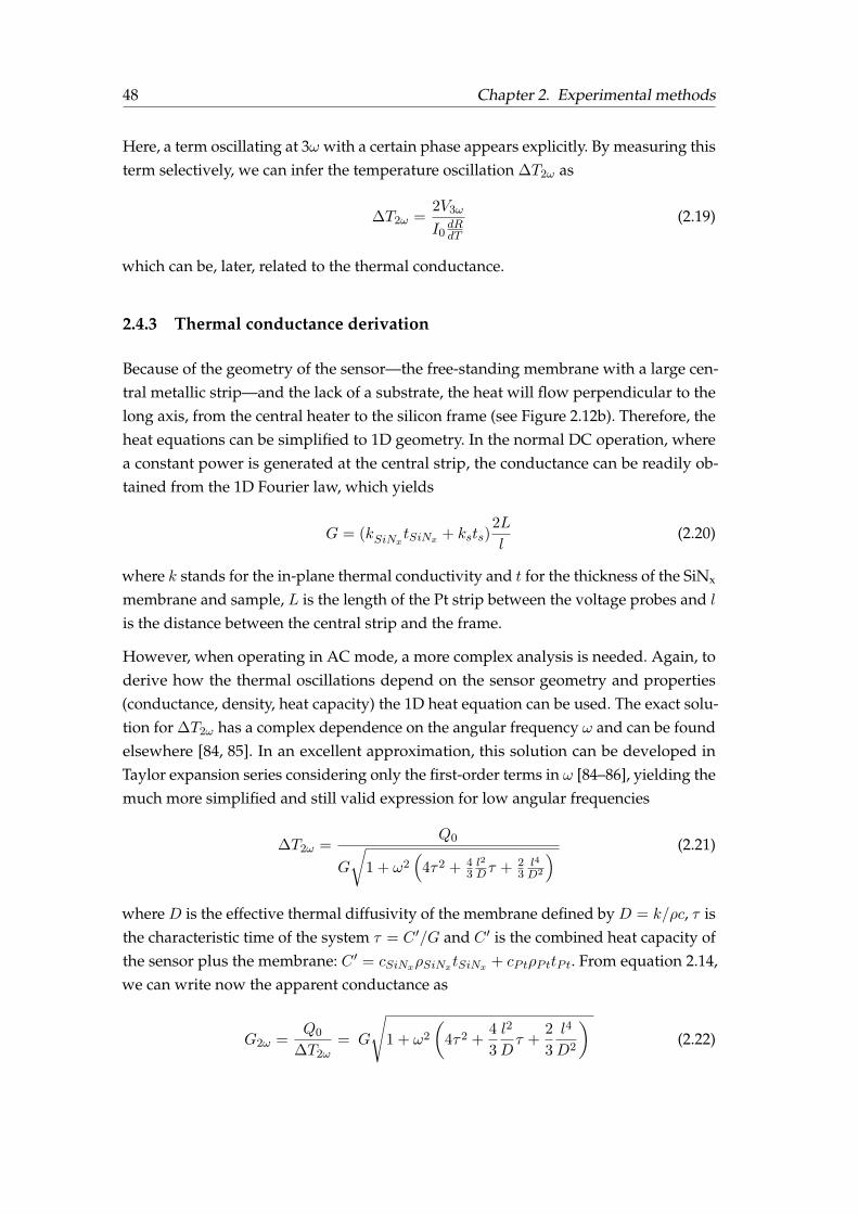
48 Chapter 2. Experimental methods
Here, a term oscillating at 3ω with a certain phase appears explicitly. By measuring thisterm selectively, we can infer the temperature oscillation ∆T2ω as
∆T2ω =2V3ω
I0dRdT
(2.19)
which can be, later, related to the thermal conductance.
2.4.3 Thermal conductance derivation
Because of the geometry of the sensor—the free-standing membrane with a large cen-tral metallic strip—and the lack of a substrate, the heat will flow perpendicular to thelong axis, from the central heater to the silicon frame (see Figure 2.12b). Therefore, theheat equations can be simplified to 1D geometry. In the normal DC operation, wherea constant power is generated at the central strip, the conductance can be readily ob-tained from the 1D Fourier law, which yields
G = (kSiNxtSiNx + ksts)
2L
l(2.20)
where k stands for the in-plane thermal conductivity and t for the thickness of the SiNx
membrane and sample, L is the length of the Pt strip between the voltage probes and lis the distance between the central strip and the frame.
However, when operating in AC mode, a more complex analysis is needed. Again, toderive how the thermal oscillations depend on the sensor geometry and properties(conductance, density, heat capacity) the 1D heat equation can be used. The exact solu-tion for ∆T2ω has a complex dependence on the angular frequency ω and can be foundelsewhere [84, 85]. In an excellent approximation, this solution can be developed inTaylor expansion series considering only the first-order terms in ω [84–86], yielding themuch more simplified and still valid expression for low angular frequencies
∆T2ω =Q0
G
√1 + ω2
(4τ2 + 4
3l2
Dτ + 23l4
D2
) (2.21)
where D is the effective thermal diffusivity of the membrane defined by D = k/ρc, τ isthe characteristic time of the system τ = C ′/G and C ′ is the combined heat capacity ofthe sensor plus the membrane: C ′ = cSiNxρSiNxtSiNx + cPtρPttPt. From equation 2.14,we can write now the apparent conductance as
G2ω =Q0
∆T2ω= G
√1 + ω2
(4τ2 +
4
3
l2
Dτ +
2
3
l4
D2
)(2.22)
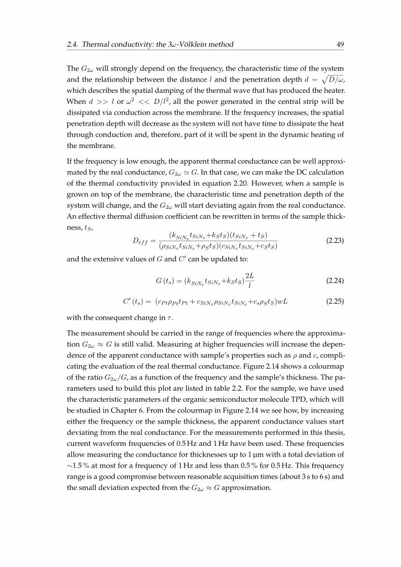
2.4. Thermal conductivity: the 3ω-Völklein method 49
The G2ω will strongly depend on the frequency, the characteristic time of the systemand the relationship between the distance l and the penetration depth d =
√D/ω,
which describes the spatial damping of the thermal wave that has produced the heater.When d >> l or ω2 << D/l2, all the power generated in the central strip will bedissipated via conduction across the membrane. If the frequency increases, the spatialpenetration depth will decrease as the system will not have time to dissipate the heatthrough conduction and, therefore, part of it will be spent in the dynamic heating ofthe membrane.
If the frequency is low enough, the apparent thermal conductance can be well approxi-mated by the real conductance, G2ω ' G. In that case, we can make the DC calculationof the thermal conductivity provided in equation 2.20. However, when a sample isgrown on top of the membrane, the characteristic time and penetration depth of thesystem will change, and the G2ω will start deviating again from the real conductance.An effective thermal diffusion coefficient can be rewritten in terms of the sample thick-ness, tS ,
Deff =(kSiNx
tSiNx+kStS)(tSiNx + tS)
(ρSiNxtSiNx+ρStS)(cSiNxtSiNx+cStS)(2.23)
and the extensive values of G and C ′ can be updated to:
G (ts) = (kSiNxtSiNx+kStS)
2L
l(2.24)
C ′ (ts) = (cPtρPttPt + cSiNxρSiNxtSiNx+csρStS)wL (2.25)
with the consequent change in τ .
The measurement should be carried in the range of frequencies where the approxima-tion G2ω ≈ G is still valid. Measuring at higher frequencies will increase the depen-dence of the apparent conductance with sample’s properties such as ρ and c, compli-cating the evaluation of the real thermal conductance. Figure 2.14 shows a colourmapof the ratio G2ω/G, as a function of the frequency and the sample’s thickness. The pa-rameters used to build this plot are listed in table 2.2. For the sample, we have usedthe characteristic parameters of the organic semiconductor molecule TPD, which willbe studied in Chapter 6. From the colourmap in Figure 2.14 we see how, by increasingeither the frequency or the sample thickness, the apparent conductance values startdeviating from the real conductance. For the measurements performed in this thesis,current waveform frequencies of 0.5 Hz and 1 Hz have been used. These frequenciesallow measuring the conductance for thicknesses up to 1 µm with a total deviation of∼1.5 % at most for a frequency of 1 Hz and less than 0.5 % for 0.5 Hz. This frequencyrange is a good compromise between reasonable acquisition times (about 3 s to 6 s) andthe small deviation expected from the G2ω ≈ G approximation.

50 Chapter 2. Experimental methods
Figure 2.14: Colourmap of the ratio between the G2ω and the GDC as a function of thefrequency and the thickness of an organic TPD sample, in this case. This Figure has been
generated using equation 2.22 and the parameters listed in table 2.2.
Parameter/material Pt SiNx TPD layer
k [W m−1 K] 33 2.65 0.16cp [J kg−1 K−1] 133 700 1000ρ [kg m−3] 21450 3180 1080
Table 2.2: Parameters used to calculate theG2ω dependence on frequency and mass shownin Figure 2.14.
2.4.4 Measurement procedure
Samples are deposited using PVD directly on the membrane without the need of ashadow mask. The thermal conductance of the system membrane/sample at a giventemperature is measured several times (50 to 100) and subsequently averaged to obtainenough statistics. Figure 2.15 shows an example of the V1ω (both from the sample andthe reference) and V3ω signals, with the latter having, essentially, the 3ω contributiondue to the good cancellation of the primary 1ω signal. Further details on the specificprocedure to obtain the conductance of the sample films are given directly in Chapter6.

2.4. Thermal conductivity: the 3ω-Völklein method 51
Figure 2.15: The different signals generated for the 3ω–Völklein measurements. The differ-ential voltage contains basically the V3ω signal due to almost total cancellation of the V1ωsignal. The data from the Figure is simulated and does not correspond to a real measure-
ment.
2.4.5 3ω technique: out of plane measurements
In this work, we have also used the well-established 3ω technique to gain access toout-of-plane (k⊥) of thin films and, in this way, complement the data of the k‖ obtainedwith the 3ω–Völklein. We briefly present here the basic details of this specific technique.
As stated before, this technique is also based on the measurement of the V3ω signal gen-erated by the self-heating of the metallic element, which allows obtaining the tempera-ture rise of the strip (∆T ). What differs this method from the 3ω–Völklein technique isthe geometry. In this case, we have a long and narrow strip on top of the sample filmwe want to measure, as sketched in Figure 2.12a. As long as the half-width of the strip(w) is much larger than the thickness of the film (tfilm), the heat flows from the heaterto the substrate almost perpendicularly. Because of this approximation and simplifiedgeometry, the contribution to the temperature rise of the strip of the film can be simplywritten as [74]
∆Tfilm =Q0
kfilm
tfilm2wL
(2.26)
where L is the length of the strip (also much larger than its thickness). The film isplaced, on top of a substrate—silicon in this case. In fact, this method was initiallydeveloped and used to measure the bulk thermal conductivity [80]. The contributionof the substrate, which also contributes to the temperature amplitude of the strip, canbe cancelled out by measuring with and without the thin film using the same sensor

52 Chapter 2. Experimental methods
Figure 2.16: Optical image of the 3ω sensor deposited using a shadow mask on top of a150 nm thick film of the organic semiconductor molecule TPD. The two big square pads
are the voltage probes; the current pads are left out the picture.
and frequency.
Sensor deposition
Here we have used as substrate monocrystalline silicon with a 450 nm silicon nitridefilm on top of it to act as a dielectric insulating layer to prevent current leakage fromthe sensor to the substrate. TPD samples are evaporated on top of the SiNx layer.Contrary to the 3ω–Völklein, the sample needs now to be removed from the chamber toevaporate the sensor on top of it in a different setup. A reference substrate (silicon plusSiNx) is also prepared. The deposition of the sensor is performed using shadow masksto shape its geometry (Figure 2.7). The sensor is evaporated by e-beam deposition andconsists of an adhesion layer of 10 nm Ti together with a 100 nm Au layer. Figure 2.16shows an optical microscope image of the strip and the two pads for the voltage probes.This method produces sensors with subtle differences in both thickness and width ofthe strip which requires further corrections of the measured data, as explained in thefollowing Section. The nominal dimensions of the evaporated sensor are L = 1 mm,2w = 5 µm and a thickness of 100 nm.
Sensor correction
Since the sensors can be slightly different, a direct subtraction between the sampleand reference temperature amplitudes cannot be performed. A different thickness and

2.5. Microfabrication, data acquisition and calibration 53
width of the strip will affect the resistance of the strip and therefore, the injected powerQ0 if the measurements are performed at a fixed current. A different width of the sensorwill also affect the Si bulk and the SiNx layer contribution to the temperature amplitude.To obtain the equivalent ∆Tref , its value has to be scaled to the geometry of the samplesensor. A more detailed procedure of this correction can be found elsewhere [85].
The 3ω measurements performed in this work (see Chapter 6) required high precisionto resolve minor differences in k⊥ of the samples. For this reason, the geometry of thesensors needs to be well-characterised. The width of the sensors was measured byAFM with a precision of ±100 nm.
2.5 Microfabrication, data acquisition and calibration
2.5.1 Device microfabrication
The microfabrication process for the nanocalorimeter is schematically described inFigure 2.17. The fabrication starts with a double-sided polished p-type silicon wafer.First, a 50 nm silicon oxide film is grown by thermal oxidation (a). The second stepconsists in growing a 180 nm thick film of low-stressed silicon nitride layer by low-pressure chemical vapour deposition (b). Then, square windows at the backside ofthe chip are opened using combined standard photolithography and reactive etchingtechniques (c), leaving exposed the underlying silicon. Now, on the front side, themetallic elements—meander-shaped circuit and electrodes—are deposited (d). Finally,a window is opened in the backside by KOH anisotropic etching of the Si layer (e)with the bottom silicon nitride window defining its area. This last process will opena cavity with a trapezoidal cross-section and a free-standing silicon membrane layer.More details on the microfabrication process can be found elsewhere [78, 79].
The sample must be placed selectively only on the sensing area, so the temperature pro-file is not disturbed and an accurate measurement can be performed. This is achievedby using microfabricated silicon shadow masks (as shown in the sketched Figure 2.7).These masks self-align due to the same window geometry as the chip, guaranteeingthe well-adjustment between the sensing area and the mask’s window. In this way, theevaporation area is completely delimited when preparing the sample with a physicalvapour deposition method.
The microfabrication process of the 3ω–Völklein devices is relatively similar to thenanocalorimeter devices. More details on the specific followed steps can be foundelsewhere [85].
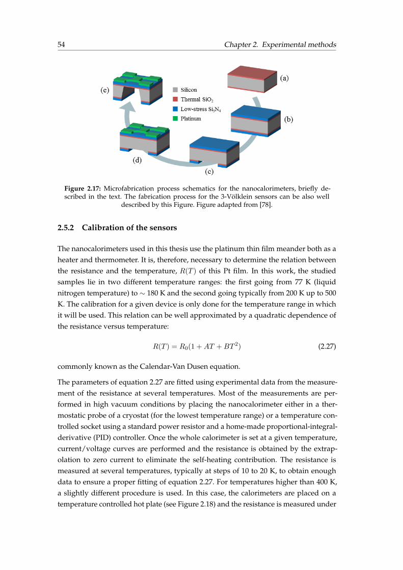
54 Chapter 2. Experimental methods
Figure 2.17: Microfabrication process schematics for the nanocalorimeters, briefly de-scribed in the text. The fabrication process for the 3-Völklein sensors can be also well
described by this Figure. Figure adapted from [78].
2.5.2 Calibration of the sensors
The nanocalorimeters used in this thesis use the platinum thin film meander both as aheater and thermometer. It is, therefore, necessary to determine the relation betweenthe resistance and the temperature, R(T ) of this Pt film. In this work, the studiedsamples lie in two different temperature ranges: the first going from 77 K (liquidnitrogen temperature) to ∼ 180 K and the second going typically from 200 K up to 500K. The calibration for a given device is only done for the temperature range in whichit will be used. This relation can be well approximated by a quadratic dependence ofthe resistance versus temperature:
R(T ) = R0(1 +AT +BT 2) (2.27)
commonly known as the Calendar-Van Dusen equation.
The parameters of equation 2.27 are fitted using experimental data from the measure-ment of the resistance at several temperatures. Most of the measurements are per-formed in high vacuum conditions by placing the nanocalorimeter either in a ther-mostatic probe of a cryostat (for the lowest temperature range) or a temperature con-trolled socket using a standard power resistor and a home-made proportional-integral-derivative (PID) controller. Once the whole calorimeter is set at a given temperature,current/voltage curves are performed and the resistance is obtained by the extrap-olation to zero current to eliminate the self-heating contribution. The resistance ismeasured at several temperatures, typically at steps of 10 to 20 K, to obtain enoughdata to ensure a proper fitting of equation 2.27. For temperatures higher than 400 K,a slightly different procedure is used. In this case, the calorimeters are placed on atemperature controlled hot plate (see Figure 2.18) and the resistance is measured under

2.5. Microfabrication, data acquisition and calibration 55
Figure 2.18: Setup for the high-temperature range calibration. The calorimeters are placedon a hot plate that is resistively heated.
argon at near-ambient pressure conditions to ensure temperature homogeneity. Theadvantage of this setup is that the connections are mechanical through the metallicrods (Figure 2.18) and the temperature of the hot plate can be raised higher than 400K. In this case, the self-heating of the heater/sensor at low currents can be neglecteddue to the excellent heat conduction through the surrounding gas, which prevents thetemperature rise. Figure 2.19 shows how the combined results of R(T ) using both ap-proaches exhibit a perfect agreement in the common temperature range explored. Theinset shows the melting of a 130 nm indium film used as a benchmark for the calibra-tion. The onset of the peak is found at (429± 1) K, in agreement the 429.75 K meltingtemperature for this material.
The 3ω–Völklein microchips are calibrated following a similar proceeding as the nano-calorimeters. In this case, the important parameter to know is the dR/dT coefficient,needed to calculate the ∆T2ω (see equation 2.19) between the central platinum stripand the silicon frame. This coefficient is obtained from the polynomial fit of the R(T )
curve and subsequent derivative. The temperature of the whole device is set using thetemperature socket (Figure 2.4).
2.5.3 Electronics and data acquisition
The same electronics (schematically shown in Figure 2.20) can be used for the fast-scanning nanocalorimetry setup, the 3ω–Völklein and the conventional 3ω. In , twotwin calorimeters are. The voltage drop in both sensors (sample and reference) is pre-amplified using the low-noise instrumental amplifiers INA 114 to fit the DAQ systemvoltage range (±10 V). The gain of the instrumental amplifiers can be finely adjustedto offer an even higher cancellation of the differential signal. Then, this voltage can
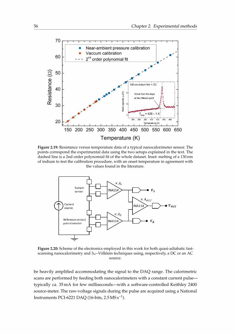
56 Chapter 2. Experimental methods
Figure 2.19: Resistance versus temperature data of a typical nanocalorimeter sensor. Thepoints correspond the experimental data using the two setups explained in the text. Thedashed line is a 2nd order polynomial fit of the whole dataset. Inset: melting of a 130 nmof indium to test the calibration procedure, with an onset temperature in agreement with
the values found in the literature.
Figure 2.20: Scheme of the electronics employed in this work for both quasi-adiabatic fast-scanning nanocalorimetry and 3ω–Völklein techniques using, respectively, a DC or an AC
source.
be heavily amplified accommodating the signal to the DAQ range. The calorimetricscans are performed by feeding both nanocalorimeters with a constant current pulse—typically ca. 35 mA for few milliseconds—with a software-controlled Keithley 2400source-meter. The raw-voltage signals during the pulse are acquired using a NationalInstruments PCI-6221 DAQ (16-bits, 2.5 MS s−1).

2.5. Microfabrication, data acquisition and calibration 57
In a very similar way as we do in nanocalorimetry, one of the key points of the 3ω-based techniques is that a differential measurement permits to heavily amplify the3ω voltage coming from the sample which is, generally, small. Two sensors are usedagain, a sample and a reference, fed in series with a current wave of known intensityby a Keithley 6221. To measure only the 3ω contribution from the sample sensor, themembrane from the reference sensor is not freed from the bulk silicon. Therefore, theself-heating is completely suppressed due to the excellent thermal link between theheater and the substrate and no V3ω signal is generated. In such a way, the 1ω signalis cancelled out between both sensors and the V3ω component is only produced in thesample sensor. The reference sensor can be substituted by a simple potentiometer toadjust the cancellation of the 1ω.
The same acquisition system used for the nanocalorimetry setup is also used for the3ω–Völklein and 3ω, although at lower acquisition frequencies. The used time windowcorresponds to three current periods, which is translated into nine periods for the V3ωcomponent. Using LabView software, a discrete Fourier transform is performed, so theamplitude and phase of the signals in 1ω and 3ω are extracted. Once the sample deviceis calibrated, the ∆T2ω and, subsequently, G, can be obtained using equations 2.19 and2.20.


Chapter 3
Stability of physicalvapour-deposited glasses
3.1 Introduction
As we advanced in the Introduction chapter, one of the advantages of physical vapourdeposition is the possibility to tailor the stability of the glass by tuning the depositionconditions. Briefly, when the substrate temperature is around 0.85 times the glass tran-sition temperature, the vapour-deposited glasses, also dubbed ultrastable glasses (UG),exhibit enhanced properties, such as low enthalpy [28, 29, 56], high kinetic stability [29,35], low heat capacities [35, 69] or high density [39, 45].
In this chapter, we use fast-scanning nanocalorimetry to obtain the specific heat signa-ture of the glass transition in VD glasses grown at different deposition temperatures.Nanocalorimetry allows access to several properties of the evaporated organic amor-phous layers. For instance, the thermodynamic stability of a glass can be quantifiedusing the limiting fictive temperature, calculated by integration of the specific heatcurve [21]. Here, three glass-formers of two different natures are used. The first stud-ied material is the organic solvent toluene, which is taken as a model glass former.Ultrastable glasses of toluene have been prepared and characterized by several groups.At GNaM, we had previously characterized VD toluene glasses using the fast-scanningnanocalorimetry technique [29, 30]. Those studies already demonstrated the growthof glassy films with much higher onset temperatures and lower enthalpies than theliquid-cooled glasses. Ishii et al. [46, 87] used laser-light interference techniques to mea-sure the specific volume of these glasses and showed its dependence on depositiontemperature. Ahrenberg at al. [35] and Bhattacharya et al. [53] used, respectively ACchip-calorimetry and fast scanning calorimetry (using a filament as a heater/sensor)and measured the kinetic and thermodynamic stability of glasses deposited at differenttemperatures. Smith et al. [43] used inert gas permeation to proof also the stability ofthese glasses.

60 Chapter 3. Stability of physical vapour-deposited glasses
The nanocalorimetry technique and data analysis have been refined since the firststudies performed at GNaM [29]. Therefore, the present study on toluene films aims togain further insights into the main mechanisms governing the formation of VD glassesthanks to the improvement of the technique, a feature that will be further explored inChapter 4.
The other two studied glass-formers are the organic semiconductor molecules TPDand α-NPD, both solid at room temperature, with their glass transition at 333 K and368 K, respectively. In a recent work from Dalal et al. [45], both TPD and α-NPD werealready shown to form denser glasses—and thus, more stable—when evaporated atthe temperature window of 0.8-0.9Tg.
Regardless of the different nature between toluene and the two organic semiconductormolecules, their behaviour with respect to their glass-forming ability is fairly similar.Hence, the results concerning the three materials are displayed and discussed in paral-lel throughout this chapter. The thermodynamic and kinetic stabilities are studied as afunction of the deposition conditions through the specific heat trace of the devitrifica-tion.
3.2 Stability of vapour-deposited glasses
The properties of VD glasses strongly depend on the deposition conditions. From theanalysis of the specific heat curves corresponding to glasses deposited at differenttemperatures, information on both kinetic and thermodynamic stability is obtained fortoluene, TPD and α-NPD. However, the deposition temperature is not the only factorcontrolling the stability of the evaporated glasses. The stability is always a compromisebetween the molecular mobility at the surface, provided by the substrate temperaturethat will also set the maximum stability attainable, and the time that the moleculeshave to explore their best configuration before being buried into the bulk, which willbe determined by the deposition rate. When the deposition rates are as low as 0.5-1 nm s−1 or below, the stability is not largely affected by this factor. Hence, in this study,we focus only on the deposition temperature effect on the glass stability for a fixeddeposition rate—generally, below 0.5 nm s−1.
3.2.1 Toluene
Thin film glasses, between 20 and 250 nm thick, of toluene of different stabilities areprepared by changing the substrate temperature (Tdep) between 82 K (0.71Tg) and 135 K(1.15Tg) at a growth rate of 0.32 nm s−1. Figure 3.1 shows the calorimetric trace for filmsof toluene of equal thickness but deposited at six substrate temperatures, together with
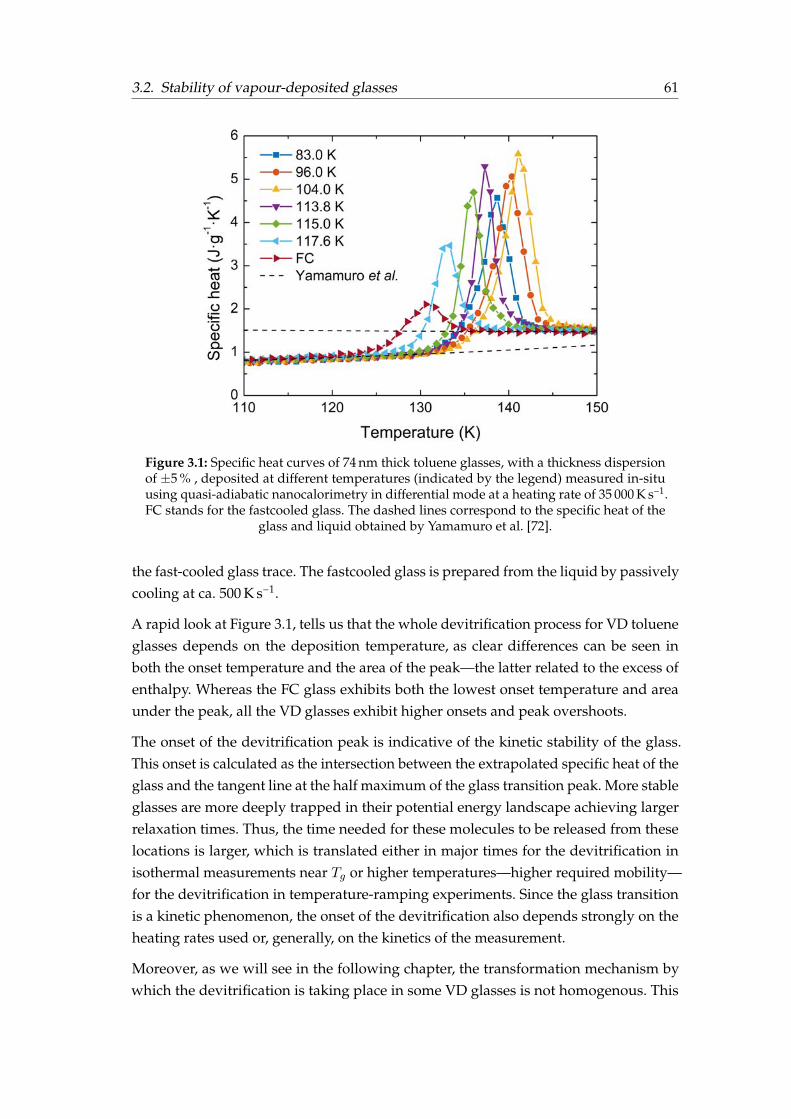
3.2. Stability of vapour-deposited glasses 61
Figure 3.1: Specific heat curves of 74 nm thick toluene glasses, with a thickness dispersionof ±5 % , deposited at different temperatures (indicated by the legend) measured in-situusing quasi-adiabatic nanocalorimetry in differential mode at a heating rate of 35 000 K s−1.FC stands for the fastcooled glass. The dashed lines correspond to the specific heat of the
glass and liquid obtained by Yamamuro et al. [72].
the fast-cooled glass trace. The fastcooled glass is prepared from the liquid by passivelycooling at ca. 500 K s−1.
A rapid look at Figure 3.1, tells us that the whole devitrification process for VD tolueneglasses depends on the deposition temperature, as clear differences can be seen inboth the onset temperature and the area of the peak—the latter related to the excess ofenthalpy. Whereas the FC glass exhibits both the lowest onset temperature and areaunder the peak, all the VD glasses exhibit higher onsets and peak overshoots.
The onset of the devitrification peak is indicative of the kinetic stability of the glass.This onset is calculated as the intersection between the extrapolated specific heat of theglass and the tangent line at the half maximum of the glass transition peak. More stableglasses are more deeply trapped in their potential energy landscape achieving largerrelaxation times. Thus, the time needed for these molecules to be released from theselocations is larger, which is translated either in major times for the devitrification inisothermal measurements near Tg or higher temperatures—higher required mobility—for the devitrification in temperature-ramping experiments. Since the glass transitionis a kinetic phenomenon, the onset of the devitrification also depends strongly on theheating rates used or, generally, on the kinetics of the measurement.
Moreover, as we will see in the following chapter, the transformation mechanism bywhich the devitrification is taking place in some VD glasses is not homogenous. This
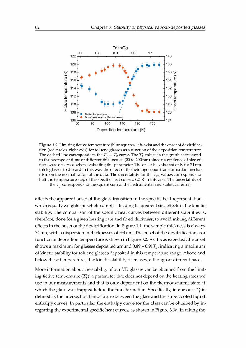
62 Chapter 3. Stability of physical vapour-deposited glasses
Figure 3.2: Limiting fictive temperature (blue squares, left-axis) and the onset of devitrifica-tion (red circles, right-axis) for toluene glasses as a function of the deposition temperature.The dashed line corresponds to the T ′f = Tg curve. The T ′f values in the graph correspondto the average of films of different thicknesses (20 to 200 nm) since no evidence of size ef-fects were observed when evaluating this parameter. The onset is evaluated only for 74 nmthick glasses to discard in this way the effect of the heterogeneous transformation mecha-nism on the normalisation of the data. The uncertainty for the Ton values corresponds tohalf the temperature step of the specific heat curves, 0.5 K in this case. The uncertainty of
the T ′f corresponds to the square sum of the instrumental and statistical error.
affects the apparent onset of the glass transition in the specific heat representation—which equally weights the whole sample—leading to apparent size effects in the kineticstability. The comparison of the specific heat curves between different stabilities is,therefore, done for a given heating rate and fixed thickness, to avoid mixing differenteffects in the onset of the devitrification. In Figure 3.1, the sample thickness is always74 nm, with a dispersion in thicknesses of ±4 nm. The onset of the devitrification as afunction of deposition temperature is shown in Figure 3.2. As it was expected, the onsetshows a maximum for glasses deposited around 0.89 – 0.91Tg, indicating a maximumof kinetic stability for toluene glasses deposited in this temperature range. Above andbelow these temperatures, the kinetic stability decreases, although at different paces.
More information about the stability of our VD glasses can be obtained from the limit-ing fictive temperature (T ′f ), a parameter that does not depend on the heating rates weuse in our measurements and that is only dependent on the thermodynamic state atwhich the glass was trapped before the transformation. Specifically, in our case T ′f isdefined as the intersection temperature between the glass and the supercooled liquidenthalpy curves. In particular, the enthalpy curve for the glass can be obtained by in-tegrating the experimental specific heat curves, as shown in Figure 3.3a. In taking the

3.2. Stability of vapour-deposited glasses 63
(a) Enthalpy versus temperature (b) T ′f versus thickness
Figure 3.3: (a) Limiting fictive temperature determination for ca. 130 nm thick layers oftoluene deposited at different temperatures, as labelled in the legend. The FC stands forthe fastcooled glass. The enthalpic curves for the different samples are obtained by inte-grating the specific heat with respect to the temperature. The dashed line corresponds tothe extrapolated supercooled liquid (SCL) enthalpy using the specific heat data from Ya-mamuro et al. [72]. The arrows indicate how the limiting fictive temperature is determinedfor each curve. (b) The limiting fictive temperature versus thickness of toluene samples fordifferent deposition temperatures, as indicated by the legend. The dashed lines correspond
to the mean value.
SCL enthalpy curve as a reference, we are assuming that the liquid phase we obtainafter the glass transition is always the same, independently on the previous thermalhistory of our glass. Contrary to the Ton, the T ′f does not depend on the transformationmechanism. T ′f does not depend either on the thickness of the films as can be seen inFigure 3.3b, at least for the deposition temperature range and thicknesses under studyfor toluene glasses.
In Figure 3.2, we represent also the limiting fictive temperature (red-circles, left-axis)together with the onset of devitrification (blue-squares, right-axis) as a function thedeposition temperature for toluene glasses. There is a high coincidence between themaximum of kinetic and thermodynamic stability, which is evidenced by a minimumin T ′f , for the deposition temperature range of 100-108 K that corresponds to 0.85-0.92Tg.The high stability range at 100 – 108 K is in agreement with previously reported resultsfrom Ahrenberg et al. [35], where they measured with AC nanocalorimetry the onsettemperature for vapour-deposited glasses of toluene at much lower heating rates of10 K min−1. The T ′f are slightly lower compared to the previously published values atGNaM [29]. This discrepancy is well-explained by the procedure they used to extractthe heat capacity data of thick films, which underestimated the enthalpy involved inthe transition leading to higher values of T ′f . See reference [30] for further details.
Another interesting feature that can be seen in Figure 3.2 is that glasses deposited be-tween 110 K and 120 K have a limiting fictive temperature that coincides with their
64 Chapter 3. Stability of physical vapour-deposited glasses
deposition temperature. In a previous work from Dalal et al. [39], it was shown thata glass deposited at substrate temperatures between ∼0.89Tg and Tg have the prop-erties expected for the supercooled liquid at that temperature, what would indicatethe equilibration to the supercooled liquid state during the deposition. In general, thelowest temperature of this equilibrium range depends on the deposition rate, i.e. forsome molecules slower deposition rates yield a smaller low-temperature limit [69]since they have more time to equilibrate. However, there is still the limit of the labo-ratory time scales even for the surface equilibration process. On the other hand, theupper boundary of this temperature range is not necessarily the conventional Tg, butit is determined by the cooling rate imposed between the deposition temperature andthe measurement temperature. It is possible to obtain glasses which are in equilibriumwith the liquid above Tg if the cooling rate is fast enough. Consequently, above thisupper-temperature limit, the stability of the resulting glass will become independentof the deposition temperature. In our case, glasses are grown in the range from 0.7to 1.15Tg (82 to 130 K) and passively cooled at a rate of ca. 500 K s−1. Cooling from ahigh temperature liquid at this rate results in a glass with a T ′f of ca. 120 K. Thus, if thedeposition temperature is higher than 120 K, the resulting glass will always have, withthis cooling rate, a T ′f of 120 K regardless of the deposition temperature, as can be seenin Figure 3.2.
3.2.2 TPD and α-NPD
A very similar study is now presented for two organic semiconductor glass-formers,from now on referred also as OSG. Now, thin layers between 20 and 200 nm are de-posited at a rate of 0.21 nm s−1 for TPD and 0.16 nm s−1 for α-NPD. The explored sub-strate temperatures in this section are in the range of 0.6-1.1Tg, being 333 K and 368 Kthe glass transition temperatures of TPD and α-NPD respectively.
Figures 3.4 for TPD and 3.5 for α-NPD show the calorimetric trace for 72 nm thickglasses of TPD and 95 nm thick glasses of α-NPD with thickness dispersion of 4 % and7 %, respectively. Similarly as we have seen for toluene, both the onset and area of thepeak clearly depend on Tdep. In both cases, the onset temperature is higher for glassesdeposited in the range of 0.85-0.9Tg. This increase in Ton is accompanied by a higherenthalpy overshoot, as described before for toluene films.
The calculation of T ′f for both TPD and α-NPD present some difficulties. The fast heat-ing rates used in this study shift the glass transition to much higher temperatures and,consequently, the SCL specific heat has to be largely extrapolated to obtain the T ′f—around 100 K in the case of both OSG. To this drawback, we have to add the lack ofspecific heat data for these materials, both in the liquid and the glass region. Small

3.2. Stability of vapour-deposited glasses 65
Figure 3.4: Specific heat curves of 72 nm thick film glasses of TPD deposited at differenttemperatures (indicated in the legend). The thickness dispersion within the samples is of
±4 %.
Figure 3.5: Specific heat curves of 95 nm thick α-NPD glasses deposited at different temper-atures (indicated by the legend). The dispersion in thickness within the different samples
is of ±7 %.
errors in the linear term of the specific heat of the SCL (quadratic in the enthalpy repre-sentation) can be largely magnified at the extrapolation. Consequently, it is not possibleto give reliable absolute data of the fictive temperatures of our samples. Despite thelack of accuracy in the determination of the supercooled liquid enthalpy, it is possible

66 Chapter 3. Stability of physical vapour-deposited glasses
Figure 3.6: Limiting fictive temperature (blue squares, left-axis) and the onset of devitrifi-cation (red circles, right-axis) for TPD glasses as a function of the deposition temperature.The T ′f is expressed as the relative change with respect to the conventional glass, Tdep = Tg ,plotted as a function of Tdep. The value at each Tdep is the mean T ′f of 20 to 200 nm thicklayers, as it is size independent for this thickness and deposition temperature range. Thedashed line correspond to a straight line with a slope of one. The uncertainty in T ′f corre-sponds to the square sum of statistical uncertainty (95 % of confidence interval) and the
instrumental uncertainty.
to distinguish with precision and reproducibility the different thermodynamic stabil-ities since the error, if any, is systematic. Keeping this in mind, we can represent thedifference T ′f − Tf,g as a function of Tdep, where Tf,g is the fictive temperature that weobtain for the glass deposited at Tg. In the case of toluene, reporting accurate valuesfor the limiting fictive temperature is possible since the extrapolation needed is onlyabout 30 to 40 K from the supercooled liquid region to the intersection with the T ′f atthe glass region. Moreover, the liquid specific heat for toluene is well reported [72].
In Figure 3.6, for TPD, and in Figure 3.7, for α-NPD, we represent the fictive tempera-ture change relative to a sample deposited at Tg, for which it is assumed that T ′f = Tg,and the onset temperature versus the deposition temperature. The dependence of thestability on Tdep is very similar to what we have seen for toluene. As we decrease thedeposition temperature starting from Tg (or above), the stability of the evaporated sam-ples increases until reaching a maximum in Ton (minimum in T ′f ) around 285 K for TPDand 315 K for α-NPD. This maximum in the thermodynamic stability coincides nowwith a deposition temperature of ∼0.85Tg for both OSG. When the deposition temper-ature is further decreased, the stability of the evaporated samples starts to decreaseagain. Despite the determination in the T ′f lacks accuracy, we can plot a straight linewith a slope of one—in analogy to what we have done for toluene—to represent the

3.3. Correlation between stability and density 67
Figure 3.7: Limiting fictive temperature (blue squares, left-axis) and the onset of devitrifica-tion (red circles, right-axis) for α-NPD glasses as a function of the deposition temperature.The T ′f is expressed as the relative change with respect to the conventional glass, Tdep = Tg ,plotted as a function of Tdep. The value at each Tdep is the mean T ′f of 20 to 200 nm thicklayers, as it is size independent for this thickness and deposition temperature range. Thedashed line corresponds to a straight line with a slope of one. The uncertainty in T ′f cor-responds to the square sum of statistical uncertainty (95 % of confidence interval) and the
instrumental uncertainty.
equilibrium SCL (dashed lines in Figures 3.6 and 3.7). We can see how the T ′f of glassesdeposited above 0.85Tg follows reasonably well this line indicating the equilibrationof these glasses to the SCL.
3.3 Correlation between stability and density
We have seen how three different molecular glass formers—toluene and the two or-ganic semiconductor molecules—exhibit a similar behaviour when comparing the sta-bility versus the deposition temperature, expressed in terms of the ratio Tdep/Tg. In allthree cases, the stability of the evaporated glasses is maximum when evaporated inthe temperature range of 0.8-0.90Tg. In what seems a universal behaviour, many othermolecular glass formers have also been reported to form ultrastable glasses when evap-orated at the same temperature window. Within them, the first systems in which thisbehaviour was reported, TNB and the pharmaceutical drug indomethacin [10]. It hasalso been reported on other pharmaceutical drugs such as celecoxib [33], in other ben-zene derivatives such as ethylbenzene [29, 30, 43, 46] or methyl-m-toluate [38], and inthe same organic semiconductors TPD and α-NPD [45].

68 Chapter 3. Stability of physical vapour-deposited glasses
The results shown in Figures 3.6 and 3.7 agree with the ones presented in Dalal et al.[45] and Walters et al. [40] for TPD and α-NPD. There, they report how these systemsshow a dependence of density on the substrate temperature. The parameter they useto characterise the glass stability is the density variation relative to the SCL. In Figures3.8a and 3.8b we plot our limiting fictive temperature data together with density dataof TPD [40] and α-NPD [45], respectively and with properly scaled axes. Both Figuresshow a good correlation between the ∆T ′f and the density variations. Regarding the α-NPD data, although there is a slight deviation at the lowest explored Tdep (the error barsfrom the reference are plotted in this case for the sake of comparison), the correlation isstill high for the 0.7-1.0Tg range in the deposition temperatures. This good correlationbetween these two quantities was already reported by Rodríguez-Tinoco et al. for themodel glass former indomethacin [54]. A resembling Figure for toluene is not shownsince there is no density data covering all Tdep range found in the literature. Both thedensity and the limiting fictive temperatures measurements shown here are propertiesaveraged over the whole sample. At the light of these results, one could say that glasseswith the same T ′f (or density) deposited below and above the 0.85Tg are structurallyequivalent. However, as we will see in Chapter 4, this equivalence does not hold truewhen looking at other glass properties. All we can say is that T ′f and density providean equivalent way of characterising the thermal stability as a function of Tdep.
(a) TPD (b) α-NPD
Figure 3.8: Comparison between the limiting fictive temperature (left-axis) and densityvariation as a function of the deposition temperature for TPD and α-NPD glasses. Density
data is taken from Wlaters et al. [40] for TPD and from Dalal et al. [45] for α-NPD
Toluene, TPD and α-NPD show the same behaviour with deposition temperature asmany other molecular glass-formers, with a maximum of stability around the 0.85Tg.Below this temperature, the stability (and density) starts to decrease again. The most ac-cepted view for the ultrastable glass formation is still the enhanced molecular mobilityon the surface [28]. Molecules at the surface are much faster in sampling their config-urational phase space than the molecules trapped in bulk—as it would happen in anageing process—reaching lower-energy configurations even achieving the correspond-ing supercooled liquid equilibrium configuration. When the deposition temperature
3.4. Summary 69
is further decreased, even the surface equilibration times become larger than the labtimescales precluding the molecules the possibility to sample their best configurationsin the potential energy landscape properly. Very recently, Ngai et al. [31] have relatedthe stable glass formation to the enhanced surface mobility and the β-relaxation. Briefly,they state that the stable glass Tdep region falls in-between the standard Tg, where theα-relaxation time is 100-1000 s, and the secondary Tg,β , where the relaxation time ofthe β-relaxation is 100-1000 s too.
3.4 Summary
We have used fast scanning quasi-adiabatic nanocalorimetry to characterise the glasstransition in toluene, TPD and α-NPD glasses obtained by physical vapour depositionat different substrate temperatures. When this temperature is set in the range of 0.80-0.90Tg, glasses with the highest stability can be obtained, compared to the conventionalglasses prepared from the liquid.
We have seen how glasses grown above ca. 0.90Tg have a limiting fictive temperaturethat corresponds to their deposition temperature. This suggests that these glasses arein equilibrium with the liquid, in agreement with previous results in indomethacinfrom density measurements and nanocalorimetry. For TPD and α-NPD, a good cor-relation between the limiting fictive temperature—or thermodynamic stability—andthe glass density has been found, in agreement with resembling results obtained forindomethacin.

Chapter 4
Heterogeneous transformationmechanism in vapour-depositedglasses
4.1 Introduction
Among outstanding properties of vapour-deposited thin film glasses, the heteroge-neous transformation mechanism by which they overcome the devitrification processinto the supercooled liquid state [34, 41, 42, 88] is, probably, the most remarkable. Thismechanism contrasts with the homogeneous transformation observed in glasses pre-pared by quenching the liquid. It has been proposed that in ultrastable glasses themolecules are so tightly packed that the transformation begins where the mobility ishigher, i.e. at surfaces and/or interfaces [27]. Experimentally, this phenomenon hasbeen seen using a variety of techniques in several systems. For instance, secondarymass ion spectrometry (SIMS) [41, 42] has been used to trace the evolution and transfor-mation into the supercooled liquid by following the evolution of deutered IMC multi-layers. A propagating transformation front has also been measured using spectroscopicellipsometry [40, 89] by modelling the optical response of vapour-deposited glassesof IMC and TPD through time during isothermal experiments. In AC-calorimetry forIMC [36], ethylbenzene and toluene [35], the propagating front has been inferred fromthe linear dependence of the transformation time with the thickness of the samples.Finally, in previous studies on IMC, we have inferred the growth front from the calori-metric trace of the devitrification using differential scanning calorimetry [34] and fast-scanning nanocalorimetry [34, 54] whereas Bhattacharya and Sadtchenko [53] identi-fied the transformation front, in toluene also, using another fast-scanning calorimetrytechnique.
Previous studies on many of the mentioned glass-formers have shown that the trans-formation rate is mainly driven by the mobility of the adjacent new formed liquid
72 Chapter 4. Heterogeneous transformation mechanism in VD glasses
layer [34, 40, 41, 88]. Specifically, for many organic glasses it has been found that thetransformation rate follows an empirical relation with τα, the α-relaxation time of thesupercooled liquid [90]:
vgr = Cτ−γα (4.1)
where C depends on the deposition conditions [54] and is independent of temperatureand −γ defines the slope of the growth front velocity as a function of the relaxationtime of the liquid in a log-log plot. Generally, in these molecular glass formers, therelaxation time of the liquid follows a VFT-type expression (equation 1.6). The relationexpressed in 4.1 was initially found for vapour-deposited glasses of IMC and TNBusing secondary ion mass spectrometry [41] in a limited temperature range around thecorresponding Tg of the material. More recently, we have shown using fast-scanningnanocalorimetry on that the same relationship holds across a very wide temperaturerange, from Tg up to 75 K above Tg, corresponding to 12 orders of magnitude in relax-ation time in the particular case of IMC [34].
One of the advantages of physical vapour deposition is the possibility to tailor thestability of the produced glass by tuning the deposition conditions. Several studieshave already shown that not only highly stable glasses transform via a heterogeneousmechanism, but, in general, vapour-deposited glasses with lower stability also start thetransformation process via a growth front [40, 54, 89]. For instance, Walters et al. [89]and Dalal et al. [89] measured, respectively, the front velocity of glasses of TPD and IMCwith different stability by ellipsometry close to ambient temperature. Rodríguez-Tinocoet al. used fast-scanning nanocalorimetry to measure the growth front velocity of IMCglasses spanning a broad range of stabilities [54]. It was found that the velocity at whichthe front propagates in glasses of different stabilities, including the ultrastable glass,had the same temperature dependence. However, the absolute value of the growthfront velocity depends on the stability of the glass. This result was in contrast withboth RFOT and pinning models, which foresee a strong temperature dependence of thegrowth front velocity but a much smaller influence of the stability [66, 91], determinedin our case by the deposition temperature.
As shown in the previous chapter, the thermodynamic stability of a glass is typi-cally quantified using the limiting fictive temperature. Several studies have concluded,though, that this parameter does not univocally determine some properties of the glass[92]. In this context, we established in a previous work [54] that the growth front veloc-ity of a transforming glass of IMC could not be determined considering only its limitingfictive temperature, but two different dependencies arose, depending on whether theglass was deposited above or below 0.85Tg. According to previous studies [39, 93, 94],IMC vapour-deposited glasses exhibit certain molecular anisotropy that depends onthe deposition conditions. From the correlation between growth front velocity andmolecular anisotropy in IMC glassy films, it was inferred that the arrangement of the

4.2. Identification of the transformation mechanism 73
molecules in the glass could also play a role in the transformation velocity. Yokoyamashowed that molecular orientation in organic glasses is directly related to the shapeof the molecules [95]; more planar or linear molecules tend to align parallel to thesubstrate at certain deposition conditions, while more bulky or compact moleculestend to have random orientation producing more isotropic glasses. Depending on thedeposition temperature, molecules can even tend to align perpendicular to the sub-strate, as was shown for different organic molecules by Dalal and co-workers [45, 93].In particular, the two organic semiconductors studied in this thesis—TPD and α-NPD—have been shown to exhibit a molecular orientation that depends on the depositionconditions [45].
In this chapter, we first present a method to identify the transformation mechanism gov-erning the glass transition in vapour-deposited glasses. Secondly, we address the vari-ables that apparently control the heterogeneous transformation mechanism of glassesprepared in a wide range of stabilities. For that purpose, we extract from the calori-metric trace corresponding to samples of toluene, TPD and α-NPD the growth frontvelocity and analyse it as a function of the different glass properties, such as thermalstability or molecular orientation.
4.2 Identification of the transformation mechanism
The specific heat curves seen in Figures 3.2, 3.6 and 3.7 are obtained by dividing the heatcapacity curve by the total mass of the film, and thus equally weighting the contributionof the whole sample during the transformation. When using this type of normalisation—i.e. the specific heat—, samples transforming via a homogeneous bulk mechanismshow a complete overlap regardless of their thickness, as in the case of the fast-cooledglass. On the other hand, if the glass transition is not a homogeneous process, massnormalisation yields curves with different onset temperatures. This is the case of ourVD films with onset temperatures that shift depending on the thickness of the sample,as shown in the left-side panels of Figures 4.1, 4.2 and 4.3 for toluene, TPD and α-NPD respectively. We had previously observed this shift for indomethacin thin filmglasses [34, 54], where this behaviour was shown to be related to the transformationmechanism [34].
An ad-hoc normalisation procedure of the heat capacity curves that considers the sur-face of the sample allows the identification of the transformation mechanism. Thisnormalisation procedure consists in separating the different contributions of the exper-imental heat capacity:
Cexpp (T ) = (m0 −ml(T ))cgp +ml(T )clp + ∆hdml(T )
dT(4.2)

74 Chapter 4. Heterogeneous transformation mechanism in VD glasses
Figure 4.1: Left panels: specific heat curves for toluene films obtained at different deposi-tion temperatures: (a) 82.6 K (0.7Tg), (b) 104.0 K (0.89Tg) and (c) 113.8 K (0.97Tg); and (d)after fast cooling the super-cooled liquid. Right panels: curves obtained by normalizingthe same heat capacity data from the left panel using equation 4.3. The legend indicates
the thickness of the films in nm.
where clp and cgp refer respectively to the specific heat capacity of the liquid and theglass, ∆h the enthalpy involved in the transformation, m0 the total mass of the sampleand ml the mass that has transformed already to the liquid, which is a function oftime and temperature and can be expressed as ml(T ) = ρl(T )Aξl(T ) where ρ is thedensity of the material, A is the surface and ξl is the film thickness that has already

4.2. Identification of the transformation mechanism 75
Figure 4.2: Left panels: specific heat curves for TPD films obtained at different depositiontemperatures: (a) 220 K (0.66Tg), (b) 285 K (0.86Tg) and (c) 334K (Tg). Right panels: curvesobtained by normalising the same heat capacity data from the left panel using equation
4.3. The legend indicates the thickness of the films.
transformed to liquid, assuming a situation where exclusively a transformation frontis taking place. Expressing equation 4.2 in terms of film thickness and moving all thepotential non-common parameters of the different samples, i.e. surface area and totalthickness, to the left side of the equation we get:
cnormp (T ) =Cexpp (T )
ρA− cgpξ0 = ξl (T )
(clp − cgp
)+ ∆h
dξl(T )
dT(4.3)
where ξ0 is the total thickness of the sample and ξl the liquid transformed fraction. Thisaccounts for the change in thickness from glass to liquid. The thicknesses are inferredfrom the mass (inferred from the cp at the liquid phase) using the density, assumedconstant, and the area, corresponding to the sensing area of the chip. The densityvalues are reported in Section 2.1.6. The model proposed in equation 4.3 allows theidentification of this heterogeneous mechanism because we have two distinct phasesduring the transformation: a fraction of the sample that has already been transformedto the supercooled liquid and a fraction that remains still a glass.
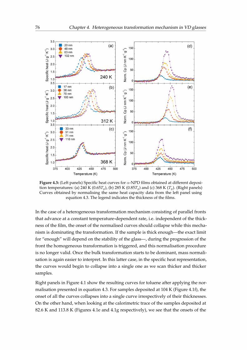
76 Chapter 4. Heterogeneous transformation mechanism in VD glasses
Figure 4.3: (Left panels) Specific heat curves for α-NPD films obtained at different deposi-tion temperatures: (a) 240 K (0.65Tg), (b) 285 K (0.85Tg) and (c) 368 K (Tg). (Right panels)Curves obtained by normalising the same heat capacity data from the left panel using
equation 4.3. The legend indicates the thickness of the films.
In the case of a heterogeneous transformation mechanism consisting of parallel frontsthat advance at a constant temperature-dependent rate, i.e. independent of the thick-ness of the film, the onset of the normalised curves should collapse while this mecha-nism is dominating the transformation. If the sample is thick enough—the exact limitfor “enough” will depend on the stability of the glass—, during the progression of thefront the homogeneous transformation is triggered, and this normalisation procedureis no longer valid. Once the bulk transformation starts to be dominant, mass normali-sation is again easier to interpret. In this latter case, in the specific heat representation,the curves would begin to collapse into a single one as we scan thicker and thickersamples.
Right panels in Figure 4.1 show the resulting curves for toluene after applying the nor-malisation presented in equation 4.3. For samples deposited at 104 K (Figure 4.1f), theonset of all the curves collapses into a single curve irrespectively of their thicknesses.On the other hand, when looking at the calorimetric trace of the samples deposited at82.6 K and 113.8 K (Figures 4.1e and 4.1g respectively), we see that the onsets of the

4.2. Identification of the transformation mechanism 77
normalised curves overlap only up to ca. 138 K and 133 K, respectively. Above that tem-perature, the bulk transformation is triggered, and the front normalization procedurestarts to underestimate the transformed volume which, in the case of homogeneousbulk processes, depends on the total mass of the sample. It is worth noticing that thenormalization procedure described by equation 4.3 does not provide any meaningfulinterpretation for the FC glass (see Figure 4.1h). In the specific heat representation, allthe curves for the FC glasses collapse into a single one, indicative of a homogenousmechanism (see Figure 4.1d).
A similar analysis can be done with the organic semiconductor molecules. Figures4.2 and 4.3 represent the specific heat (left panels) and the ad hoc normalised curves(right panels) for TPD and α-NPD, respectively. Like before, we show the calorimetrictrace for glasses deposited at three different deposition temperatures for each material,the UG glass with a Tdep around 0.85Tg, a lower stability glass the deposited around0.65Tg (left-branch of Figure 3.6 ) and a glass deposited at Tg. Glasses deposited atTg show an apparent shift in the onset of the transformation only for the thinnestsamples, approximately up to 40 nm in both materials. For thicker films, the bulk istriggered, and the specific heat curves start to collapse since the transformation takesplace homogeneously in the rest of the volume. On the other hand, glasses deposited at0.65Tg and 0.85Tg (Figures 4.2a-b and 4.3a-b) show a clear onset shift with the thicknessin the specific heat curves (left-panels) whereas the surface normalization producesthe collapse of all curves to a common onset (right-panels).
We rationalise the collapse of the calorimetric trace using the normalisation presentedin equation 4.3 (left panels of Figures 4.1, 4.2 and 4.3) with the existence of a par-allel growth front mechanism. In the proposed model we have assumed a growthfront velocity that does not depend on the sample’s thickness. Under this assumption,the curves would only collapse when this parallel growth front is the only—or thedominating—transformation mechanism. As soon as the bulk transformation mech-anism appears, the ad hoc normalisation does no longer yield a single onset of thetransformation. We can define the crossover length ξco as the distance that the propa-gation front travels before the bulk transformation is triggered. This distance stronglydepends not only on the stability of the glasses but also on the deposition tempera-ture and is further investigated in Section 4.6 for the toluene system. This combinedheterogeneous and homogeneous transformation mechanism has been observed ex-perimentally for IMC [36], TNB [96] and methyl-m-toluate [38, 90] but has also beenpredicted by simulations based on facilitated Ising models [63, 64] and random pinningmodels [66].
Finally, it is worth noticing that, while we can identify that the glasses transform via apropagating growth front, we cannot distinguish between the existence of one (surface-initiated) or two fronts (surface and interface-initiated). Contrary to other techniques

78 Chapter 4. Heterogeneous transformation mechanism in VD glasses
where the growth front is directly traced—such as SIMS [41]—, in our case the front isinferred by comparing several samples with different thicknesses that exhibit a suffi-ciently dominant growth front mechanism that allows its detection. The detection ofthe existence of one or two growth fronts using nanocalorimetry can done by usingcapping layers to block the front and subsequently analyse the calorimetric trace. Thisstrategy is further addressed in Chapter 5.
4.3 Front velocity calculation
The differential equation 4.3 can be solved for ξl(T ) using the experimental data. Thederivative of ξl(T ) is, precisely, the transformation rate of the transition (see Figure4.4a). While the dominating transformation mechanism is the surface-initiated front—as already indicated on the right side of equation 4.3—this rate can directly yield thegrowth front velocity by:
vgr (T ) = β (T )dξl(T )
dT(4.4)
where β is the instantaneous heating rate evaluated at each temperature.
The only parameter that must be imposed in solving equation 4.4 is the total excessenthalpy of the process. This parameter is obtained by imposing that the transformedliquid fraction goes from 0, at the glass region, to ξ0, which is the total thickness of thesample fully transformed into the SCL. To obtain the front velocity, we must multiplyit by the heating rate. The latter, due to the nature of the technique, is temperaturedependent and can be readily obtained from the raw data. It is important to note thatthe growth front velocity is taken from the temperature range where all the curves—corresponding to different thicknesses and a given deposition temperature—collapse(Figure 4.4b). The velocity values for the common range are subsequently averagedamong the different thicknesses.
The range in which the propagating front can be calculated is limited, therefore, by theamount of sample that transforms via this mechanism before the bulk is triggered. Inthat framework, once the homogeneous transformation starts, the curves do no longercollapse when using the ad hoc normalisation and the vgr values cannot be obtained.We have to note that for both OSG the low accuracy of our specific heat data for bothmaterials might lead, as happened with the limiting fictive temperature, to less accurateabsolute values of the front velocity. It is important to remark that high precision isreached anyway with relative values.
Figure 4.5 shows the growth front velocity for the three thin-film glass-formers withthicknesses between 20 and 200 nm obtained at different deposition temperatures.Clearly, a change in the deposition temperature yields a glass with a different front
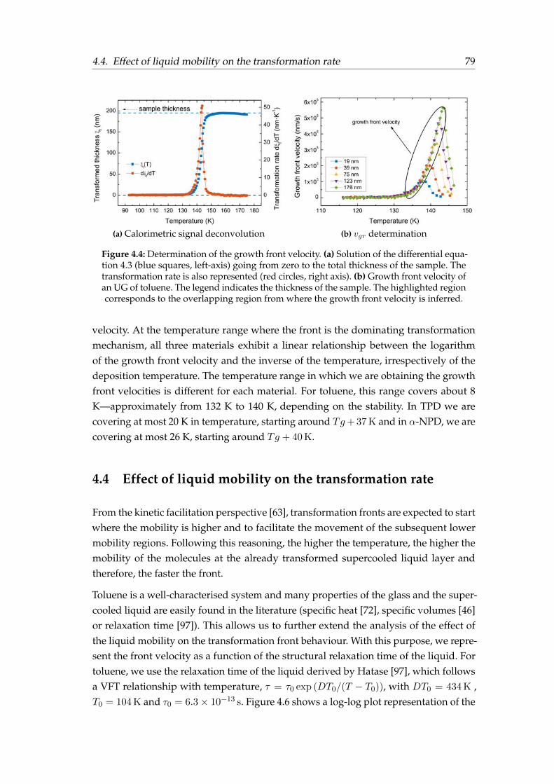
4.4. Effect of liquid mobility on the transformation rate 79
(a) Calorimetric signal deconvolution (b) vgr determination
Figure 4.4: Determination of the growth front velocity. (a) Solution of the differential equa-tion 4.3 (blue squares, left-axis) going from zero to the total thickness of the sample. Thetransformation rate is also represented (red circles, right axis). (b) Growth front velocity ofan UG of toluene. The legend indicates the thickness of the sample. The highlighted regioncorresponds to the overlapping region from where the growth front velocity is inferred.
velocity. At the temperature range where the front is the dominating transformationmechanism, all three materials exhibit a linear relationship between the logarithmof the growth front velocity and the inverse of the temperature, irrespectively of thedeposition temperature. The temperature range in which we are obtaining the growthfront velocities is different for each material. For toluene, this range covers about 8K—approximately from 132 K to 140 K, depending on the stability. In TPD we arecovering at most 20 K in temperature, starting around Tg+ 37 K and in α-NPD, we arecovering at most 26 K, starting around Tg + 40 K.
4.4 Effect of liquid mobility on the transformation rate
From the kinetic facilitation perspective [63], transformation fronts are expected to startwhere the mobility is higher and to facilitate the movement of the subsequent lowermobility regions. Following this reasoning, the higher the temperature, the higher themobility of the molecules at the already transformed supercooled liquid layer andtherefore, the faster the front.
Toluene is a well-characterised system and many properties of the glass and the super-cooled liquid are easily found in the literature (specific heat [72], specific volumes [46]or relaxation time [97]). This allows us to further extend the analysis of the effect ofthe liquid mobility on the transformation front behaviour. With this purpose, we repre-sent the front velocity as a function of the structural relaxation time of the liquid. Fortoluene, we use the relaxation time of the liquid derived by Hatase [97], which followsa VFT relationship with temperature, τ = τ0 exp (DT0/(T − T0)), with DT0 = 434 K ,T0 = 104 K and τ0 = 6.3× 10⁻¹³ s. Figure 4.6 shows a log-log plot representation of the
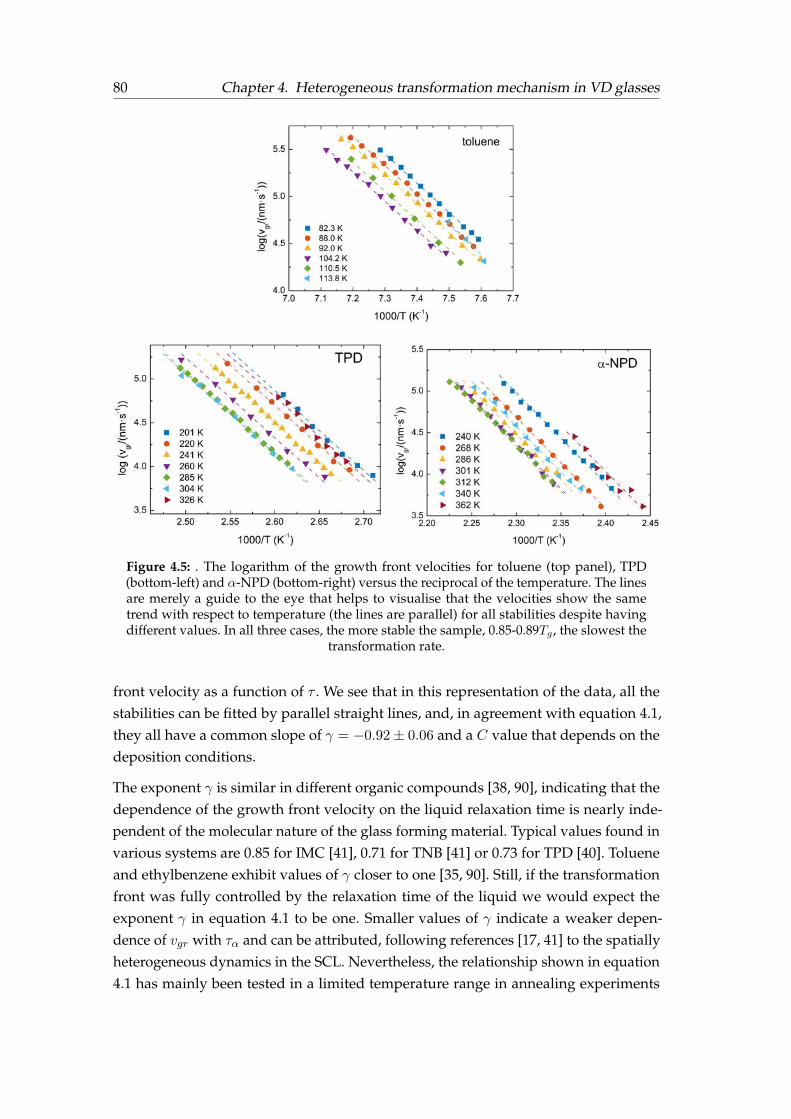
80 Chapter 4. Heterogeneous transformation mechanism in VD glasses
Figure 4.5: . The logarithm of the growth front velocities for toluene (top panel), TPD(bottom-left) and α-NPD (bottom-right) versus the reciprocal of the temperature. The linesare merely a guide to the eye that helps to visualise that the velocities show the sametrend with respect to temperature (the lines are parallel) for all stabilities despite havingdifferent values. In all three cases, the more stable the sample, 0.85-0.89Tg , the slowest the
transformation rate.
front velocity as a function of τ . We see that in this representation of the data, all thestabilities can be fitted by parallel straight lines, and, in agreement with equation 4.1,they all have a common slope of γ = −0.92± 0.06 and a C value that depends on thedeposition conditions.
The exponent γ is similar in different organic compounds [38, 90], indicating that thedependence of the growth front velocity on the liquid relaxation time is nearly inde-pendent of the molecular nature of the glass forming material. Typical values found invarious systems are 0.85 for IMC [41], 0.71 for TNB [41] or 0.73 for TPD [40]. Tolueneand ethylbenzene exhibit values of γ closer to one [35, 90]. Still, if the transformationfront was fully controlled by the relaxation time of the liquid we would expect theexponent γ in equation 4.1 to be one. Smaller values of γ indicate a weaker depen-dence of vgr with τα and can be attributed, following references [17, 41] to the spatiallyheterogeneous dynamics in the SCL. Nevertheless, the relationship shown in equation4.1 has mainly been tested in a limited temperature range in annealing experiments
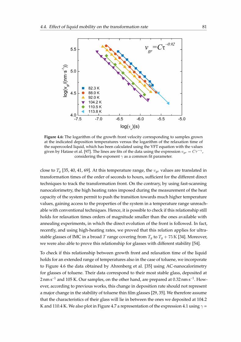
4.4. Effect of liquid mobility on the transformation rate 81
Figure 4.6: The logarithm of the growth front velocity corresponding to samples grownat the indicated deposition temperatures versus the logarithm of the relaxation time ofthe supercooled liquid, which has been calculated using the VFT equation with the valuesgiven by Hatase et al. [97]. The lines are fits of the data using the expression vgr = Cτ−γ ,
considering the exponent γ as a common fit parameter.
close to Tg [35, 40, 41, 69]. At this temperature range, the vgr values are translated intransformation times of the order of seconds to hours, sufficient for the different directtechniques to track the transformation front. On the contrary, by using fast-scanningnanocalorimetry, the high heating rates imposed during the measurement of the heatcapacity of the system permit to push the transition towards much higher temperaturevalues, gaining access to the properties of the system in a temperature range unreach-able with conventional techniques. Hence, it is possible to check if this relationship stillholds for relaxation times orders of magnitude smaller than the ones available withannealing experiments, in which the direct evolution of the front is followed. In fact,recently, and using high-heating rates, we proved that this relation applies for ultra-stable glasses of IMC in a broad T range covering from Tg to Tg + 75 K [34]. Moreover,we were also able to prove this relationship for glasses with different stability [54].
To check if this relationship between growth front and relaxation time of the liquidholds for an extended range of temperatures also in the case of toluene, we incorporateto Figure 4.6 the data obtained by Ahrenberg et al. [35] using AC-nanocalorimetryfor glasses of toluene. Their data correspond to their most stable glass, deposited at2 nm s−1 and 105 K. Our samples, on the other hand, are prepared at 0.32 nm s−1. How-ever, according to previous works, this change in deposition rate should not representa major change in the stability of toluene thin film glasses [29, 35]. We therefore assumethat the characteristics of their glass will lie in between the ones we deposited at 104.2K and 110.4 K. We also plot in Figure 4.7 a representation of the expression 4.1 using γ =

82 Chapter 4. Heterogeneous transformation mechanism in VD glasses
Figure 4.7: The logarithm of the front velocity as a function of temperature for toluenesamples deposited at 104.2 and 110.4 K and at a deposition rate of 0.35 nm s−1. Dashed redand yellow lines correspond to the fit of the data shown in panel figure 4.6 extended tolower temperatures. Star symbols correspond to data obtained by Ahrenberg et al. [35]using AC-calorimetry at low temperatures. Ahrenberg’s films were grown at 2 nm s−1 andat a deposition temperature of 105 K. The continuous grey line is a representation of theexpression vgr = Cτ−γ using γ = 0.92 and a prefactor C that fits both our 104.2 and 110.4K data and the 105 K data from Ahrenberg et al., using a line width of around ±13 %. Theblack dashed line corresponds to two independent Arrhenius fits for the high and lowtemperature data shown. The inset shows the same data but as a function of the relaxation
time of the liquid.
0.92 and a prefactor C that fits both our 104.2 and 110.4 K data and the 105 K data fromAhrenberg et al. [35] within a tolerance of ±13 %. Considering this uncertainty, wecan see a good match of our high-temperature data and Ahrenberg’s low-temperaturedata, spanning the relationship between liquid relaxation time and front velocity up toTg + 25 K, equivalent to eight orders of magnitude in relaxation time. We want to re-mark that an Arrhenius relation would not fit both the low and high-temperature data,as can be seen in Figure 4.7. There, we see how different activation energies would benecessary to fit the two sets of data.
Still, our technique cannot distinguish between the existence of one or two fronts, com-ing from the surface and the interface with the substrate, and thus, our growth rate val-ues can differ up to a factor 2 when compared with those obtained by other techniquesthat can differentiate the evolution of single fronts [42]. Some novel strategies canbe employed to infer the simultaneous existence of one or two fronts in temperature-ramping experiments, such as using a lower mobility materials as a capping layer,which will be shown in Chapter 5. However, this strategy was not straightforwardapplicable to the case of toluene analysed here.

4.5. Effect of glass properties on the transformation rate 83
Our lack of accurate specific heat data for TPD and α-NPD precludes us to perform asimilar analysis on these two materials. However, in the case of TPD, Walters et al. [40]calculate the activation energy—fitting an Arrhenius equation—for the transformationfront propagation rate which we can use to compare with the values we obtain. There,as in our case, the front velocity dependence on temperature seems independent of thedeposition temperature. In their case, the average activation energy for their surface-initiated front is of (380± 20) kJ mol−1. In a similar way, from our data in Figure 4.5 forTPD we can extract the activation energy:
Ea = −R log e∂ log vgr∂(1/T )
(4.5)
where R is the universal gas constant. Thus, the average activation energy we obtainfor our data is (176± 10) kJ mol−1, which is the mean value of the slope obtained fromindependent linear fits of the different deposition temperatures.
Our activation energy value differs from the reported value in Ref. [40], about a factorof 2. However, again, we must consider that we are comparing the front velocity withintwo completely different temperature regimes. Transformation front velocity data byWalters et al. [40] is obtained through isothermal measurements at Tg + 13 K at most.Our data is obtained at Tg + 40 K and above. We can look in Figure 4.7 for toluene,to provide a better picture of this mismatch. We have seen that, in a wider tempera-ture range, the growth front velocity does not follow an Arrhenius behaviour in thewhole range. Instead, the growth front velocity behaviour follows a VFT-like behaviourmediated by the structural relaxation time τα of the liquid. In that scenario, differentapparent activation energies are expected when looking at distinct temperature range.Particularly, the apparent activation energy at high temperatures is expected to besmaller than close to Tg, as seen from the slopes of the black dashed lines in Figure4.7. Since structural relaxation time of TPD follows a VFT expression [40], our loweractivation energy is consistent with a growth front velocity depending on the mobilityof the SCL via the power relationship with τα of equation 4.1.
4.5 Effect of glass properties on the transformation rate
Using fast-scanning nanocalorimetry, we find that the dependence with temperature ofthe transformation front is the same irrespective of the stability of the samples. Theseresults are in line with those of previous studies on indomethacin [54, 89] and on TPD[40]. This common dependence on temperature of the transformation front providesadditional evidence of the dominating role of the mobility of the supercooled liquidlayer on the velocity of the front. Still, glasses deposited at different temperaturestransform at distinct pace as seen from Figures 4.8a and 4.8b for the OSG and in Figure

84 Chapter 4. Heterogeneous transformation mechanism in VD glasses
Figure 4.8: Growth front velocity (relative to the slowest value, the UG) as a function ofthe deposition temperature for (a) TPD and (b) α-NPD.
4.9a for toluene (right-axis, red diamonds), where the vgr values have been expressedrelative to the slowest velocity.
For instance, toluene glasses prepared at Tdep = 82.3 K = 0.70Tg have a transformationfront that advances 3 times faster than the glass prepared at Tdep = 104.2 K = 0.89Tg.In fact, the most thermally stable glass shows the slower transformation front. In asimilar way, the TPD glasses prepared at Tdep = 285 K and 304 K—corresponding to0.86Tg and 0.91Tg. Figure 4.9a exhibits the slowest transformation front, up to five tosix times slower than the ones prepared at Tdep = 201 K (0.60Tg). α-NPD behaves inthe same way, with the most stable glasses presenting the lower front velocities (Figure4.8b).
As we have seen in Chapter 3, the deposition temperature determines the stability ofthe PVD glasses, and a commonly used parameter to quantify this stability is the lim-iting fictive temperature. In Figure 4.9a and using a proper scaling factor, the limitingfictive temperature data has been superimposed (blue open squares, left-axis) to frontvelocity data. We can see a good agreement between both quantities. This agreementis better seen in Figure 4.9b, where the front velocity is represented versus the limitingfictive temperature, in this case, scaled as (Tg − Tf )/Tg). The different symbols fromFigure 4.9b indicate if the glasses have been grown at a deposition temperature above(squares) or below (triangles) 0.89Tg (UG). We can see that there is no significant differ-ence in growth front velocity between depositing below and above 0.89Tg and that thetransformation rate appears to be mostly determined by the thermodynamic stabilityof the glass.
These results contrast with what is observed for the organic semiconductors TPD andα-NPD, as can be seen in Figures 4.10a and 4.10b, where we directly plot the frontversus the limiting fictive temperature, making a distinction (using different symbols)for glasses deposited above and below the maximum of thermal stability, at 0.85Tg in
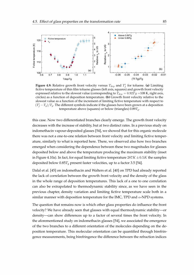
4.5. Effect of glass properties on the transformation rate 85
Figure 4.9: Relative growth front velocity versus Tdep and T ′f for toluene. (a) Limitingfictive temperature of thin film toluene glasses (left axis, squares) and growth front velocityexpressed relative to the slowest value (corresponding to Tdep = 0.92Tg =108 K, right axis,circles) as a function of deposition temperature. (b) Growth front velocity relative to theslowest value as a function of the increment of limiting fictive temperature with respect to(T ′f −Tg)/Tg . The different symbols indicate if the glasses have been grown at a deposition
temperature above (squares) or below (triangles) 0.89Tg .
this case. Now two differentiated branches clearly emerge. The growth front velocitydecreases with the increase of stability, but at two distinct rates. In a previous study onindomethacin vapour-deposited glasses [54], we showed that for this organic moleculethere was not a one-to-one relation between front velocity and limiting fictive temper-ature, similarly to what is reported here. There, we observed also how two branchesemerged when considering the dependence between these two magnitudes for glassesdeposited below and above the temperature producing the maximum stability (insetin Figure 4.10a). In fact, for equal limiting fictive temperature 287K±0.5K the samplesdeposited below 0.85Tg present faster velocities, up to a factor 3.5 [54].
Dalal et al. [45] on indomethacin and Walters et al. [40] on TPD had already reportedthe lack of correlation between the growth front velocity and the density of the glassin the whole range of deposition temperatures. This lack of a one to one correlationcan also be extrapolated to thermodynamic stability since, as we have seen in theprevious chapter, density variation and limiting fictive temperature scale both in asimilar manner with deposition temperature for the IMC, TPD and α-NPD systems.
The question that remains now is which other glass properties do influence the frontvelocity? We have already seen that glasses with equal thermodynamic stability—ordensity—can show differences up to a factor of several times the front velocity. Inthe aforementioned study on indomethacin glasses [54], we associated the emergenceof the two branches to a different orientation of the molecules depending on the de-position temperature. This molecular orientation can be quantified through birefrin-gence measurements, being birefringence the difference between the refraction indices

86 Chapter 4. Heterogeneous transformation mechanism in VD glasses
(a) TPD (b) α-NPD
Figure 4.10: Growth front velocity relative to the lowest velocity (the glass deposited at0.86Tg) is plotted as a function of (T ′f − T ′f,g)/Tg (where T ′f,g is the fictive temperaturefor the glass deposited at Tg) for both OSG. The square points correspond to samples de-posited below 0.86Tg, whereas the circles correspond to samples deposited above 0.86Tg.The symbol scheme is also used to distinguish between negative birefringence (orangecircle), positive (open blue squares) and zero (blue filled squares) correlating our datawith reported birefringence values from Dalal et al. [45]. The zero birefringence is consid-ered when |∆n| < 0.01. Positive birefringence data, only distinguished for α-NPD. Inset:equivalent representation for indomethacin data, adapted from Rodríguez-Tinoco et al.
[54]
∆n = nz−nxy, a direct consequence of molecular orientation and the anisotropic polar-izability tensors from these molecules. In a similar study on TPD and α-NPD [45], theorder parameter Sz—the average orientation of the long axis of the molecules to thesurface normal—is also measured from dichroism measurements and shown to scalewith birefringence (see Figure 4.11, reprinted from [45]). In this figure, three distinctthree regions (sketched in Figure 4.12) depending on the values of these parameterscan be distinguished:
(i) Negative birefringence and −0.5 < Sz < 0, associated with molecules with acertain degree of horizontal orientation. In Figure 4.11, negative birefringencevalues and Sz are reported for glasses deposited below ca. 0.90Tg.
(ii) Zero birefringence and Sz = 0, corresponding to isotropic molecular orientation.Glasses deposited above 0.97Tg are isotropic.
(iii) Positive birefringence and 0 < Sz < 1, associated with molecules that tend toorient vertically. Those glasses deposited between 0.90Tg and 0.97Tg show smallpositive values of birefringence and Sz .
To perform a similar analysis on TPD and α-NPD, our front velocity data is also rep-resented in Figure 4.10a considering birefringence data from Figure 4.11 [45] on thesetwo molecules. Although birefringence is a good indicator of the anisotropy of the
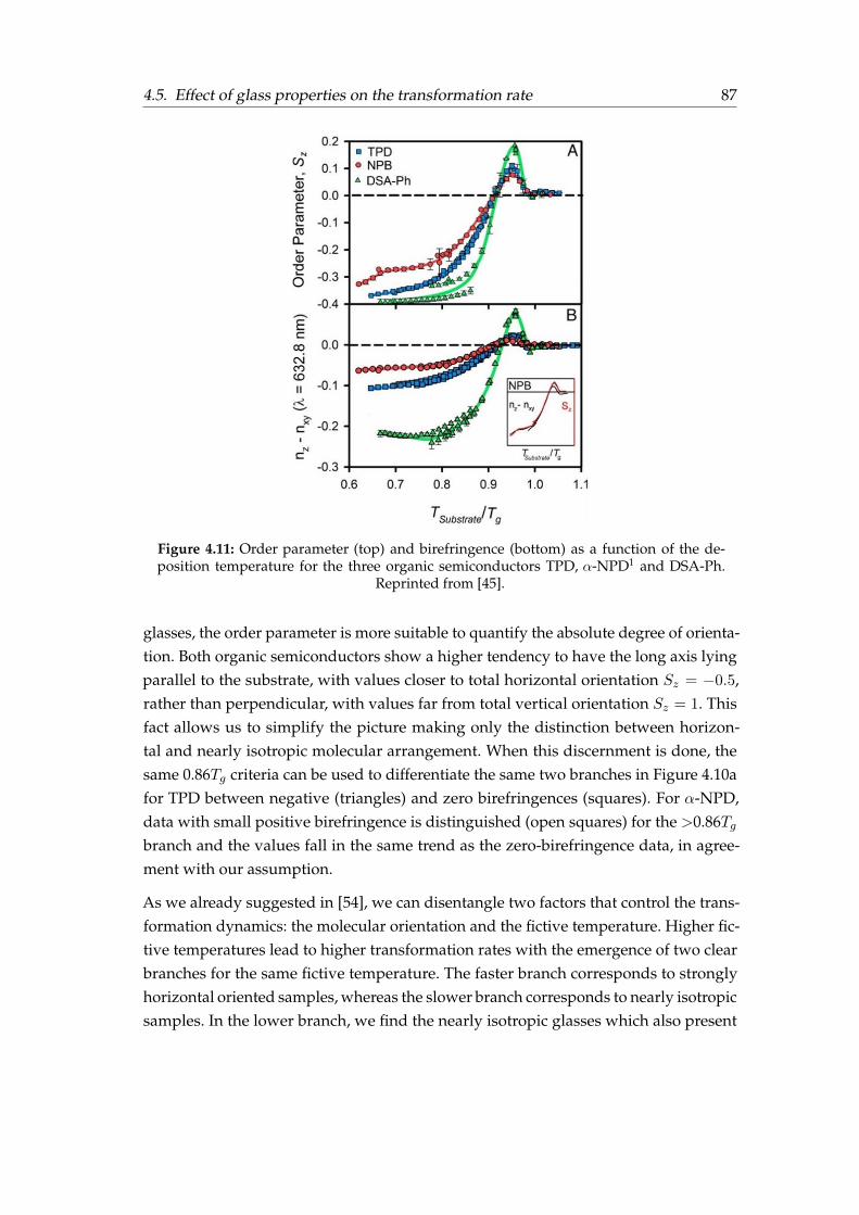
4.5. Effect of glass properties on the transformation rate 87
Figure 4.11: Order parameter (top) and birefringence (bottom) as a function of the de-position temperature for the three organic semiconductors TPD, α-NPD1 and DSA-Ph.
Reprinted from [45].
glasses, the order parameter is more suitable to quantify the absolute degree of orienta-tion. Both organic semiconductors show a higher tendency to have the long axis lyingparallel to the substrate, with values closer to total horizontal orientation Sz = −0.5,rather than perpendicular, with values far from total vertical orientation Sz = 1. Thisfact allows us to simplify the picture making only the distinction between horizon-tal and nearly isotropic molecular arrangement. When this discernment is done, thesame 0.86Tg criteria can be used to differentiate the same two branches in Figure 4.10afor TPD between negative (triangles) and zero birefringences (squares). For α-NPD,data with small positive birefringence is distinguished (open squares) for the >0.86Tgbranch and the values fall in the same trend as the zero-birefringence data, in agree-ment with our assumption.
As we already suggested in [54], we can disentangle two factors that control the trans-formation dynamics: the molecular orientation and the fictive temperature. Higher fic-tive temperatures lead to higher transformation rates with the emergence of two clearbranches for the same fictive temperature. The faster branch corresponds to stronglyhorizontal oriented samples, whereas the slower branch corresponds to nearly isotropicsamples. In the lower branch, we find the nearly isotropic glasses which also present

88 Chapter 4. Heterogeneous transformation mechanism in VD glasses
Figure 4.12: Schematic representation in 2D of three possible molecular arrangements(horizontal, isotropic, and vertical) and the parameters used in reference [45] to quantify
it. Sz is the order parameter and ∆n the birefringence.
clearly different transformation velocities. In the latter case, the fictive temperature—or density—dominates the growth front, with the less stable glasses—or less dense—being the ones exhibiting faster velocities. In the faster branch, this discrimination isnot so clear, as lower deposition temperatures yield both less stable glasses and morehorizontally oriented molecules.
Is this picture of non-isotropic molecular packing consistent with our observations intoluene? Although not symmetrical, the toluene molecule has indeed a much loweraspect ratio than TPD or α-NPD. If molecular orientation played a role in the velocityof the front, the absence or a small contribution of anisotropy would result in a transfor-mation rate that would only depend on the stability of the glass, which is indeed whatwe can see in Figure 4.9b for toluene. WAXS measurements by Ishii et al. [98] on tolueneglasses deposited at 0.89Tg show a small anisotropic peak, which they associate to theformation of particular dimers more energetically favourable. However, the presenceof these dimers does not imply necessarily that toluene molecules tend to align with apreferred orientation when deposited at different temperatures. According to previouswork from Yokoyama et al. [95], small or no preferred orientation should be expectedfrom a small molecule such as toluene. If this was the case, and no other parametersapart from molecular orientation and thermodynamic stability—or density—wouldplay a role in determining the front velocity, then we would see a perfect correlationbetween front velocity and limiting fictive temperature, as in toluene.
4.6 Crossover length in toluene glasses
Up to now, we have focused our attention on the heterogeneous front-like transforma-tion. However, as we have seen, if the samples are thick enough, the homogeneoustransformation is eventually activated and will start dominating the transformationfor increasing thicknesses.
We can define the crossover length, ξco as the distance travelled by the front before thehomogeneous mechanism dominates the transformation. This distance can be infered

4.6. Crossover length in toluene glasses 89
Figure 4.13: Position of the maximum of the glass transition peak as a function of thethickness of the film. The legend indicates the deposition temperature of the correspondingglasses. Samples with similar limiting fictive temperature have been plotted with the sametype of symbol and colour. Void symbols correspond to glasses deposited above 0.89Tg andfilled symbols to glasses obtained below 0.89Tg . The curves are vertically shifted for clarity.Experimental data are fitted with an arbitrary function as a guide to the eye (continuousline). The dashed line provides an estimation of the position of the maximum of the glass
transition peak once the homogeneous transformation mechanism dominates.
from the calorimetric specific heat curves. When the homogeneous transformation isthe dominating mechanism, the glass transition simultaneously occurs in the remain-ing volume of the sample, and therefore, the transformed fraction is basically propor-tional to the total mass. In this way, if glasses are thicker than the crossover length, themass normalised specific heat curves show a temperature value of the maximum ofthe glass transition peak that remains constant, independent of their thickness. A clearexample of this tendency is found in Figures 4.1a and 4.1c. We can, therefore, infer thecrossover length by representing the position of the maximum of the glass transitionpeak as a function of the thickness of the films. While there is a temperature shift ofthe peak position, the heterogeneous mechanism will still have a significant impacton the transformation. Figure 4.13 shows the position of the maximum of the glasstransition peak as a function of the thickness of the films for toluene glasses grown atdifferent deposition temperatures. The curves have been vertically shifted for clarity.To facilitate the interpretation of the results we have plotted the glasses with similar fic-tive temperature with the same symbol and colour. Data from glasses deposited above0.89Tg are plotted using void symbols, and we have used filled symbols for glassesdeposited below this temperature.

90 Chapter 4. Heterogeneous transformation mechanism in VD glasses
Irrespective of the deposition temperature the position of the glass transition peakshifts to higher temperatures as thickness increases and tends to stabilise at a certainthickness where bulk transformation sets in. As a guide to the eye, the different datasets from Figure 4.13 have been fitted with the same function. We can use the derivativeof this function to provide a rough estimation of the crossover length. Considering theasymptotic nature of the function, we have defined the crossover length as the thicknessat which the derivative of the function is equal to 0.002 K nm−1, i.e. when the changein the position of the glass transition peak is equal to a 0.2 %. Table 4.1 summarises thecalculated values of crossover length together with the corresponding deposition andlimiting fictive temperatures.
The first conclusion one can extract from the Figure 4.13 is that the crossover lengthdepends strongly on the deposition temperature. Glasses deposited between 0.75 and0.90Tg, corresponding to the range of deposition temperatures for maximum stability[29, 30, 35] in toluene, achieve thicker crossover lengths. For higher and lower deposi-tion temperatures, the homogeneous transformation mechanism starts at lower temper-atures, dominating the transformation before the front has travelled a longer distance.In a previous study, Bhattacharya et al. found that stable toluene glasses transformedvia a front mechanism up to thicknesses of around 2 µm [53]. With our technique, weare limited in film thickness, so it is not possible for us to determine the crossoverlength maximum for stable glasses.
Tdep [K] 82.6 88.0 92.2 104.0 110.8 111.6 112.6 113.8 115.0Tdep/Tg 0.706 0.752 0.788 0.888 0.947 0.953 0.962 0.972 0.982
T ′f [K] 114.7 113.8 112.6 110.0 110.9 112.3 113.0 113.9 114.8
ξco [nm]200 >200 >200 >200 200 200 115 77 53±30 ±30 ±30 ±30 ±30 ±20
Table 4.1: Limiting fictive temperature, T ′f , and cross-over length, ξco, for samples de-posited at different substrate temperatures, Tdep. The cross-over length has been estimatedas the thickness for which the variation of the position of the glass transition peak is onlyof 0.2 %. The uncertainty has been determined from propagation of the fitting functionand the uncertainty in the fitting parameters. The uncertainty in deposition and limiting
fictive temperature is ±0.5 K.
Although we do not see variations in the growth front velocity between glasses grownat different deposition temperatures but encoded with the same limiting fictive tem-perature, we do observe remarkable changes in their crossover lengths. The crossoverlength depends on the velocity of the front but also on the dynamics of the transfor-mation mechanism in the remaining volume of glass [64, 66]. If the front velocity isunivocally determined by T ′f , as our data in Figure 4.13 suggests, but the crossoverlength is not, then in the case of toluene the homogeneous transformation will not bedetermined by T ′f alone. In particular, glasses deposited at 115.0 K and 82.6 K having

4.6. Crossover length in toluene glasses 91
T ′f = (114.7± 0.5) K, transform via a heterogeneous mechanism up to ca. 50 nm and200 nm, respectively, while having similar front velocities. Since, as we have definedit, the crossover length represents the length that the front propagates before the bulktransformation dominates, the variation of crossover length can be related to a changein the onset temperature of the bulk glass. It is important to emphasise that the limitingfictive temperature provides information on the average stability of the glass and it hasbeen previously shown that T ′f and density, both of them average magnitudes, show agood correlation [54] (see Figure 3.8).
The intriguing question is: why two glasses with comparable average stability mayshow different onset temperatures for the bulk transformation? In the ongoing debateabout what happens to the relaxation time below Tg, there are some studies that revealtwo equilibration time scenario [99, 100]. Cangialosi et al. [99] in a recent study aboutthe enthalpy recovery in polymers aged at low temperatures for extended periods oftime reported the existence of two relaxation mechanisms. According to these authors,the differences in the formation of the glass would be reflected in their devitrificationbehaviours. Extrapolating their results, we speculate that it may be the case that glassesdeposited well below Tg are densified by a different mechanism compared with thosedeposited close to Tg, at the equilibrium line. This hypothesis could explain the differ-ent devitrification temperatures for glasses with the same limiting fictive temperaturebut deposited close or far from Tg. Data from Figure 4.13 can be further analysed usingthis new perspective. The dependence of fictive temperature with deposition tempera-ture is clearly different on both sides of the minimum. While close to Tg the dependenceis strong, a milder dependence can be observed at lower temperatures. Considering thedivergence of relaxation times at temperatures close to T0 (T0 = 104 K for toluene [97]),a much stronger dependence on the limiting fictive temperature should be expectedfor glasses deposited below 0.89Tg, unless a different mechanism would dominate theformation of the glass. We are cautious since this interpretation seems to be in contrastwith recent results from Zhang et al. [101], which show complete decoupling betweensurface and bulk dynamics. Enhanced surface mobility with respect to bulk appears tobe the origin of the high stability of vapour-deposited glasses [27, 44]. Still, it is worthnoting that a small difference of 2 K in the onset temperature would already producethe observed differences in crossover length for glasses with the same T ′f . A deeperunderstanding of the bulk transformation mechanism in toluene stable glasses as afunction of the deposition temperature is needed to extract further conclusions.
92 Chapter 4. Heterogeneous transformation mechanism in VD glasses
4.7 Summary
We have seen how the first stages of the transformation of vapour-deposited glassesinto the supercooled liquid state correspond to a heterogeneous mechanism, in partic-ular, to a supercooled liquid parallel front that starts at the surface of the sample. Thetransformation mechanism can be readily identified by an appropriate analysis of thecalorimetric trace of the devitrification. As has been demonstrated for other organicmolecules, the propagation velocity of this transformation front is strongly dominatedby the mobility of the supercooled liquid molecules. We have shown, specifically fortoluene, how a linear relation holds between the logarithm of the front velocity andthe logarithm of the relaxation time of the liquid for an extended temperature range,covering eight orders of magnitude in relaxation time.
While the most thermodynamically stable glasses present the slowest transformationrates, we have identified two different behaviours when trying to correlate the growthfront velocity with the stability of the PVD glasses. For toluene, the front velocity cor-relates with the limiting fictive temperature and seems enough to determine the frontvelocity. However, in both organic semiconductors, the thermodynamic stability is notsufficient to explain the difference in the front velocities, leading to the appearance oftwo different relations between front velocity and limiting fictive temperature.
Molecular orientation could play a role in the way the molecules are incorporated inthe liquid layer, as previous observations in vapour-deposited glasses of indomethacinhave suggested. In this context, we can speculate that the differences observed betweentoluene and the two organic semiconductors are related to the different geometry ofthese molecules. While TPD and α-NPD present anisotropic molecular packing de-pending on the deposition temperature, the simplicity and low aspect ratio of thetoluene molecule could preclude a strong molecular orientation in the films. In thisway, only thermodynamic stability and equivalently density, would conditionate thetransformation rate.
The stability however does not determine all the features observed for the glass tran-sition in toluene glasses. Considerable differences in the crossover length can be seenfor glasses with the same thermal stability but prepared at different deposition tem-peratures. Although this behaviour could be related to the existence of two distinctmechanisms of glass formation at temperatures close and far from Tg, a thorough anal-ysis of the homogeneous (bulk) glass transition in a large deposition temperature rangewould be necessary to confirm or refute this hypothesis.
Chapter 5
Homogeneous transformationmechanism in vapour-depositedglasses
5.1 Introduction
We have seen how we can effectively produce highly stable glasses by vapour de-positing them at the appropriate substrate temperature. Although the thermodynamicstability of an ultrastable glass cannot be significantly enhanced within experimentaltime scales, as it already has the properties of an equivalent hyper-aged glass [28],the kinetic stability of these glasses is dominated by the surface-initiated growth frontmechanism they exhibit. For instance, a 20 nm thick layer of an ultrastable glass willtake one-fifth less time to fully transform into supercooled liquid than a 100 nm thicklayer at the same annealing temperature. Thus, the heterogeneous transformation caneventually dynamite the high stability achieved for these glasses. This represents themajor limitation for the conceivable applications of the UG. The amount of time at agiven temperature these glasses can endure before transforming to the supercooledliquid is what will, in the end, determine the practical applications they can be usedfor.
The transformation into the supercooled liquid of stable glasses is expected to beginat surfaces, where the mobility is higher. It can be free surfaces [26, 27], but also in-terfaces with a more mobile material, for instance, a layer of conventional glass [41].Also, a slower propagating front starting at the interface with the substrate has beenidentified for TPD and IMC using spectroscopic ellipsometry during an isothermalannealing protocol [40, 89]. The transformation of stable glasses into the supercooledliquid can be elucidated in terms of the kinetic facilitation concept. That is, the idea thatan immobile region can become mobile only if mobility is present in an adjacent region
94 Chapter 5. Homogeneous transformation mechanism in VD glasses
[102]. Facilitated kinetic Ising models have already been successfully used to repro-duce the behaviour of ultrastable glasses, more specifically, in predicting the constantvelocity growth front [63, 64]. Hence, adopting the facilitated kinetics point of view,we can think of further manipulating the properties of the previously studied glasses.The basic idea is that if the highly-mobile surface layers are blocked—somehow—thenthe growth front transformation mechanism is suppressed. This methodology was al-ready applied by Sepúlveda et al. [88], who capped the free surface of a stable glassof indomethacin with a higher Tg stable glass and was able to avoid in this way theformation of a growth front. By eliminating—apparently—the surface mobility, theyincreased the samples’ kinetic stability by further delaying the transformation into thesupercooled liquid.
An application field especially interested in increasing the thermal stability of vapourdeposited amorphous thin films is the OLED industry. There, two or more thin organiclayers in the range of tenths of nanometres thick are commonly used for building theelectronic devices, all of them being generally in their glassy state. The glassy layersin OLED devices do not have any free surfaces, and therefore, their thermal stabilitywill be determined by the layer with the lowest Tg material, among other factors [8,103]. The layer with the lowest Tg will have either an interface capped by the electrodelayer and the other by a higher Tg material or both interfaces covered with higher Tgmaterials, depending on the architecture of the device. Thus, it is of vital importancefor this field to understand the effect of capping on the thermal stability of organicsemiconductor glassy layers.
To carry out this study, we have chosen the organic semiconductor TPD, as it hasbeen already characterised as a function of Tdep and has been shown to be a glassformer with enhanced stability. To eliminate the surface mobility, we must choose amaterial with lower mobility, i.e. a material with a higher Tg. The chosen material isanother organic semiconductor named TCTA, with its Tg at 424 K, 91 K above the glasstransition temperature of TPD.
We characterise, as the first step, the thermal stability of TCTA as a function of depo-sition temperature since, when evaporated as a capping layer at a given depositiontemperature, its glass properties could condition the capping properties of the film.Secondly, we will study the effect of positioning the capping layer at the top, or bottom,or on both sides of the glassy film under evaluation. In this way, we will explore theimpact of this extra low-mobility layer on the transformation mechanism of the TPDglasses. Moreover, we will vary the deposition temperature of the TPD glasses to studythe homogeneous transformation in glasses with different stability.
For this study, we use the experimental setup described in Section 2.1. Briefly, we usea UHV chamber equipped with two effusion cells, which allow creating multilayers oftwo organic materials without breaking the vacuum. Samples are deposited directly

5.2. Stability of the TCTA 95
onto the calorimeter membrane which is fed with a constant intensity to keep it ata given temperature. The TPD samples are grown at (0.08± 0.01) nm s-1 and TCTAsamples at (0.07± 0.01) nm s-1. Once the corresponding multilayer is fully deposited,the nanocalorimetric temperature scan is performed as usual (see Chapter 2).
5.2 Stability of the TCTA
TCTA is an organic semiconductor molecule than yields a glass layer when evapo-rated below Tg. Figure 5.1 shows the nanocalorimetric trace for single TCTA layersdeposited at different temperatures. The heat capacity curves have been normalisedusing equation 4.3 in order to account for the apparent onset shift due to the heteroge-neous transformation mechanism, as explained in Section 4.2. The TCTA also exhibitsa calorimetric trace typical of a propagating front transformation, inferred from theapparent onset shift that the calorimetric trace exhibits as a function of the sample’sthickness (curves not shown). The onset of the devitrification, seen in the inset of Fig-ure 5.1, is taken as the onset of the front and is analogous to comparing the onsets ofsamples with different thickness, as done previously in Chapter 3. Figure 5.1 reflects asimilar behaviour to what we have seen for TPD, α-NPD and toluene as well as whathave been reported for many other organic glass formers found in literature (see Sec-tion 1.2), i.e. a clear dependence of the stability on the deposition temperature, with amaximum of stability around 0.85Tg. In this case, this maximum of both kinetic andthermodynamic stability corresponds to a substrate temperature around 360 K.
5.3 Capping configurations
Now, we want to study the impact that adding a TCTA layer in different configurationshas on the devitrification of TPD thin films. Figure 5.2 shows the four configurationswe analyse. First and for comparison purposes, we will prepare single layers of TPD(Figure 5.2a). The second step is to evaluate the effect of having one single TCTA layereither between substrate and TPD (Figure 5.2b) or capping the free surface exposed tothe vacuum (Figure 5.2c). The final configuration is to deposit TCTA layers to coverboth sides of the TPD film (Figure 5.2d).
The glass transition temperature of conventional TPD glasses is 27 K below the deposi-tion temperature that yields the most stable form of TCTA. Therefore, we are limited todeposition temperatures located at the left branch of the inset from Figure 5.1. To main-tain the experiment as simple as possible, we evaporate the capping layers of TCTAalways at the same temperature—regardless of the deposition temperature of the TPDsample. For simplicity, this temperature is chosen to be 285 K, which corresponds to the
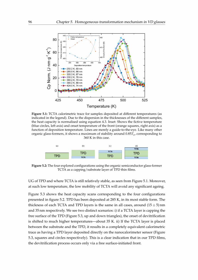
96 Chapter 5. Homogeneous transformation mechanism in VD glasses
Figure 5.1: TCTA calorimetric trace for samples deposited at different temperatures (asindicated in the legend). Due to the dispersion in the thicknesses of the different samples,the heat capacity is normalised using equation 4.3. Inset: Shows the fictive temperature(blue circles, left axis) and onset temperature of the front (orange squares, right axis) as afunction of deposition temperature. Lines are merely a guide-to-the-eye. Like many otherorganic glass-formers, it shows a maximum of stability around 0.85Tg, corresponding to
360 K in this case.
Figure 5.2: The four explored configurations using the organic semiconductor glass-formerTCTA as a capping/substrate layer of TPD thin films.
UG of TPD and where TCTA is still relatively stable, as seen from Figure 5.1. Moreover,at such low temperature, the low mobility of TCTA will avoid any significant ageing.
Figure 5.3 shows the heat capacity scans corresponding to the four configurationspresented in figure 5.2. TPD has been deposited at 285 K, in its most stable form. Thethickness of each TCTA and TPD layers is the same in all cases, around (15± 5) nmand 35 nm respectively. We see two distinct scenarios: i) if a TCTA layer is capping thefree surface of the TPD (Figure 5.3, up and down triangles), the onset of devitrificationis shifted to much higher temperatures—about 35 K. ii) If the TCTA layer is placedbetween the substrate and the TPD, it results in a completely equivalent calorimetrictrace as having a TPD layer deposited directly on the nanocalorimeter sensor (Figure5.3, squares and circles respectively). This is a clear indication that in our TPD films,the devitrification process occurs only via a free surface-initiated front.

5.3. Capping configurations 97
Figure 5.3: Heat capacity scans of the ultrastable glass of TPD for the different configura-tions presented in figure 5.2 as indicated in the legend. The thickness of the TCTA layers isof 17 nm. The thickness of the single TPD layer is 44 nm and of 34 nm for the TPD/TCTA,
TCTA/TPD and TCTA/TPD/TCTA configurations.
We now look at the TCTA calorimetric trace. In the single TCTA scan, we see thedevitrification around 460 K for a 15 nm thick layer (Figure 5.3, open squares). However,when TCTA is deposited in contact with a TPD layer, we do not see the calorimetrictrace corresponding to its devitrification (Figure 5.3, triangles and circles). A betterinsight to this phenomenon can be found in Figure 5.4, where we plot the heat capacityof the TCTA/TPD/TCTA configuration for TPD samples deposited at 0.85Tg and at Tgtogether with the previous single scan of TCTA. The calorimetric trace of the sampledeposited at Tg exhibits two well-defined transitions. The first one is the expectedtransition for TPD deposited at Tg, the second one corresponds to the devitrificationof the TCTA occurring at much lower temperatures than the expected for a singleTCTA layer, around 30 K below. Therefore, it seems likely that in the case of the cappedultrastable glass of TPD, both devitrifications—TPD and TCTA—are fully overlapped.That can also explain the slight differences in the onset and the area seen between theTCTA/TPD/TCTA configuration and the single top-capping layer. The double massof TCTA transforming in the sandwich configuration with respect to the TPD layeroverlapped with the glass transition of TPD. In fact, when looking at the curves fromthe configuration TCTA/TPD (Figure 5.3 circles), we can infer a small peak just afterthe devitrification of the TPD sample, around 430 K, which would correspond to thetransformation the 15 nm TCTA layer.
The differences between the TCTA devitrification temperatures when arranged as asingle layer or following a multilayer configuration with TPD can initially be explainedfrom the kinetic facilitation point of view. A TCTA vapour deposited layer will start
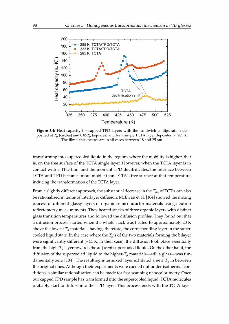
98 Chapter 5. Homogeneous transformation mechanism in VD glasses
Figure 5.4: Heat capacity for capped TPD layers with the sandwich configuration de-posited at Tg (circles) and 0.85Tg (squares) and for a single TCTA layer deposited at 285 K.
The films’ thicknesses are in all cases between 18 and 25 nm.
transforming into supercooled liquid in the regions where the mobility is higher, thatis, on the free surface of the TCTA single layer. However, when the TCTA layer is incontact with a TPD film, and the moment TPD devitrificates, the interface betweenTCTA and TPD becomes more mobile than TCTA’s free surface at that temperature,inducing the transformation of the TCTA layer.
From a slightly different approach, the substantial decrease in the Ton of TCTA can alsobe rationalised in terms of interlayer diffusion. McEwan et al. [104] showed the mixingprocess of different glassy layers of organic semiconductor materials using neutronreflectometry measurements. They heated stacks of three organic layers with distinctglass transition temperatures and followed the diffusion profiles. They found out thata diffusion process started when the whole stack was heated to approximately 20 Kabove the lowest Tg material—having, therefore, the corresponding layer in the super-cooled liquid state. In the case where the Tg’s of the two materials forming the bilayerwere significantly different (∼55 K, in their case), the diffusion took place essentiallyfrom the high-Tg layer towards the adjacent supercooled liquid. On the other hand, thediffusion of the supercooled liquid to the higher-Tg materials—still a glass—was fun-damentally zero [104]. The resulting intermixed layer exhibited a new Tg in betweenthe original ones. Although their experiments were carried out under isothermal con-ditions, a similar rationalisation can be made for fast-scanning nanocalorimetry. Onceour capped TPD sample has transformed into the supercooled liquid, TCTA moleculesprobably start to diffuse into the TPD layer. This process ends with the TCTA layer

5.4. Transformation mechanisms in capped glasses 99
intermixed with the newly formed layer, still glassy, with a depressed Tg with respectto TCTA. Despite diffusion processes in a heating ramp are slightly more complicated,this simple physical picture can explain the depressed Tg we observe for a TCTA layerin contact with a lower Tg material.
5.4 Transformation mechanisms in capped glasses
Although TPD layers do not show major differences in their devitrification process forthe configurations TCTA/TPD/TCTA and TCTA/TPD/substrate, to reduce the num-ber of factors controlling the devitrification we will continue our study with the fullsandwich configuration. In this way, the TPD layers will have two identical interfacesas substrate and top layers.
Figure 5.3 shows how the devitrification of the TPD layer is delayed when the sur-face is capped, but the transformation mechanism of TPD under this configurationremains to be confirmed. As already mentioned when explaining how to analyse thespecific heat curves of a glass transition, the transformation mechanism matters. If ahomogeneous mechanism is governing the transformation into the supercooled liquid,samples with the same stability samples but with different thicknesses should exhibita common onset—and single peak—in the specific heat curves. For that purpose, be-tween three and four thicknesses of TPD layers (approximately 20, 40, 70 and 90 nm)have been evaporated at different substrate temperatures both as single layer and withthe TCTA/TPD/TCTA sandwich geometry. The capping layers of TCTA are alwaysevaporated at 285 K with thicknesses between 10 and 20 nm.
The contribution of the heat capacity of the TCTA glass is subtracted from each curveto simplify the analysis of the curves corresponding to different sample sizes. How-ever, we must consider the following aspects: i) the mass from the TCTA layer must beinferred from the QCM reading since it is not possible to deconvolute the heat capacitysignal from the TPD and TCTA layers separately. ii) The contribution of the TCTA layercannot be subtracted in the whole temperature range of the calorimetric scan. This isbecause its devitrification occurs at different temperatures depending on whether it isin its single or multilayered configuration. Therefore, in the region after the transition,the TCTA contribution cannot be properly subtracted. iii) Consequently, the normali-sation we are performing accounts neither for the area of the peak nor the specific heatin the liquid region. iv) Once the subtraction is performed, the mass of the TPD layercan be then inferred from the heat capacity in the glass region of the resulting curve,instead of using the supercooled liquid region as was used in previous measurements.This procedure yields thicknesses in agreement with the values measured by the QCMduring the evaporation.

100 Chapter 5. Homogeneous transformation mechanism in VD glasses
Figure 5.5: Calorimetric trace of ultrastable glasses of TPD deposited at 285 K for single(void symbols) and capped layers with configuration TCTA/TPD/TCTA (filled symbols).Different symbols indicate different TPD thicknesses, as labelled in the legend. The dia-monds correspond to a TPD/TCTA bilayer configuration. The dashed black lines deter-
mine the onset of devitrification for the capped layers.
In Figure 5.5 we can see the specific heat trace for three different thicknesses of a TPDglass deposited at 0.85Tg for single and capped layers. While the single layers showthe onset shift typical of heterogeneous transformations (void symbols), the onset andpeak of the capped glass collapse regardless of the sample’s thickness, indicative ofa homogeneous transformation. The small variations in the area of the peak are anartefact produced by the different TPD/TCTA mass ratios that each sample has andthat the normalisation is not considering. Equivalent results are obtained for TPD de-posited at three more temperatures. The corresponding specific heat curves are shownin Figures 5.6a, 5.6b and 5.6c for deposition temperatures of 220 K, 250 K and 325 Krespectively. These results corroborate that the transformation is taking place via ahomogeneous mechanism not only in the case of the ultrastable glass but also for lessstable glasses. From the kinetic facilitation point of view, we are, in fact, preventing thefront by arresting the higher mobility region. Previous work from Sepúlveda et al. [88]showed that the propagating transformation front of ultrastable IMC glasses could beimpeded with a capping layer of a higher Tg material, TNB in their case. There, theyused deuterated IMC layers to follow the concentration profile during an annealing atTg + 11 K. Although their capped samples eventually transformed into the SCL, thiswas accomplished at much longer times than the samples with a free surface. In ourcase instead, we use temperature-ramping experiments to prove that the growth frontcan be blocked and the glass transition delayed. For TPD, we see how not only theUG can be capped but also less stable glasses. In the light of these results with the

5.4. Transformation mechanisms in capped glasses 101
(a) Tdep = 220 K
(b) Tdep = 250 K (c) Tdep = 325 K
Figure 5.6: Calorimetric trace of VD glasses of TPD deposited at three different Tdep forsingle (void symbols) and capped layers with configuration TCTA/TPD/TCTA (filledsymbols). Different symbols indicate different TPD thicknesses, as labelled in the legends.The diamonds correspond to a TPD/TCTA bilayer configuration and pentagons to the
TCTA/TPD configuration.
system TPD/TCTA together with the ones provided by Sepúlveda et al. [88] for thesystem IMC/TNB, the capping strategy to preclude the front transformation could begeneralised to other glass-forming materials. Moreover, it provides us the opportunityto study the homogeneous transformation of very thin films.
Before continuing let’s briefly have a look at the sample that has only TCTA actingas a substrate (Figure 5.5, diamond symbols). As we have previously anticipated forthe UG, we ruled out the possibility of having two growth fronts—one starting atthe free surface and one starting at the interface sample/substrate. Having a UG ofTPD on top of a TCTA layer produces the same calorimetric trace as having a UGof TPD sample directly on the nanocalorimeter’s substrate, Figure 5.5 (diamonds). Inprinciple, we could not directly rule out the possibility of having two fronts for higheror lower deposition temperatures. As seen in the previous chapter, the growth frontvelocity of TPD glasses deposited below 0.85Tg can be up to 5 times faster than the
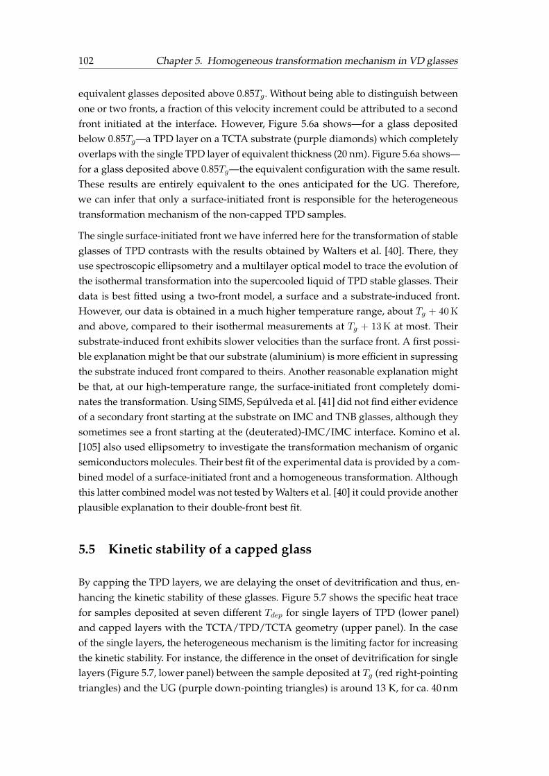
102 Chapter 5. Homogeneous transformation mechanism in VD glasses
equivalent glasses deposited above 0.85Tg. Without being able to distinguish betweenone or two fronts, a fraction of this velocity increment could be attributed to a secondfront initiated at the interface. However, Figure 5.6a shows—for a glass depositedbelow 0.85Tg—a TPD layer on a TCTA substrate (purple diamonds) which completelyoverlaps with the single TPD layer of equivalent thickness (20 nm). Figure 5.6a shows—for a glass deposited above 0.85Tg—the equivalent configuration with the same result.These results are entirely equivalent to the ones anticipated for the UG. Therefore,we can infer that only a surface-initiated front is responsible for the heterogeneoustransformation mechanism of the non-capped TPD samples.
The single surface-initiated front we have inferred here for the transformation of stableglasses of TPD contrasts with the results obtained by Walters et al. [40]. There, theyuse spectroscopic ellipsometry and a multilayer optical model to trace the evolution ofthe isothermal transformation into the supercooled liquid of TPD stable glasses. Theirdata is best fitted using a two-front model, a surface and a substrate-induced front.However, our data is obtained in a much higher temperature range, about Tg + 40 K
and above, compared to their isothermal measurements at Tg + 13 K at most. Theirsubstrate-induced front exhibits slower velocities than the surface front. A first possi-ble explanation might be that our substrate (aluminium) is more efficient in supressingthe substrate induced front compared to theirs. Another reasonable explanation mightbe that, at our high-temperature range, the surface-initiated front completely domi-nates the transformation. Using SIMS, Sepúlveda et al. [41] did not find either evidenceof a secondary front starting at the substrate on IMC and TNB glasses, although theysometimes see a front starting at the (deuterated)-IMC/IMC interface. Komino et al.[105] also used ellipsometry to investigate the transformation mechanism of organicsemiconductors molecules. Their best fit of the experimental data is provided by a com-bined model of a surface-initiated front and a homogeneous transformation. Althoughthis latter combined model was not tested by Walters et al. [40] it could provide anotherplausible explanation to their double-front best fit.
5.5 Kinetic stability of a capped glass
By capping the TPD layers, we are delaying the onset of devitrification and thus, en-hancing the kinetic stability of these glasses. Figure 5.7 shows the specific heat tracefor samples deposited at seven different Tdep for single layers of TPD (lower panel)and capped layers with the TCTA/TPD/TCTA geometry (upper panel). In the caseof the single layers, the heterogeneous mechanism is the limiting factor for increasingthe kinetic stability. For instance, the difference in the onset of devitrification for singlelayers (Figure 5.7, lower panel) between the sample deposited at Tg (red right-pointingtriangles) and the UG (purple down-pointing triangles) is around 13 K, for ca. 40 nm
5.5. Kinetic stability of a capped glass 103
thick layers. Of course, this is an apparent onset due to the heterogeneous transforma-tion mechanism and the specific heat representation of the data. This difference canbecome larger when comparing samples with different thicknesses. On the contrary,when capped, the onset difference between the same two samples is expanded up to 44K. The onset of the Tdep = Tg sample is practically the same in both cases—indicatinga small crossover length of a few nanometres. The much larger shift in the UG is in-dicative of a much higher crossover length of probably few hundreds of nanometres.Glasses with stabilities in between the ultrastable and the conventional glass showintermediate onset shifts, showing again that the crossover length is a deposition tem-perature dependent variable.
From Figure 5.7, it is worth noticing that the devitrification of the TCTA can also beseen—better discerned for the less stable samples. When visible, the glass transitionof TCTA seems to take place in all cases at the same temperature, clearly overlappingwith the transition of the UG of TPD.
In Chapter 3, we have seen how the growth front velocity does not scale with thelimiting fictive temperature—leading to the appearance of the two branches whenrepresenting the vgr(T ′f ) plot (Figure 4.10a). There, the kinetics (growth front) and thethermodynamics (T ′f ) were not completely correlated, and we invoked other glass prop-erties to explain that behaviour, such as the molecular orientation. Now that we cangain access to the bulk devitrification onset, we examine the correlation between thekinetics and thermodynamics again, i.e. Ton and T ′f . Figure 5.8 shows the onset of thebulk (left axis) and the limiting fictive temperature (right-axis) versus the depositiontemperature. The T ′f data used has been taken from Figure 3.6, since we cannot use thecapped curves to extract this value. With properly scaled axes, we see an agreementbetween both quantities within an estimated error of ±3 K. The only Tdep that seemsto fall out of the trend slightly is the glass deposited at 200 K. Ramos et al. have mea-sured the bulk calorimetric devitrification trace of VD glasses of ethylbenzene [56] andethylcyclohexane [106] with DSC at very low heating rates. They report differences inthe width of the devitrification overshoots for same T ′f glasses but deposited aboveand below the Tdep giving the maximum stability. They see that glasses deposited be-low this temperature show broader peaks than the ones deposited above the UG Tdep.When analysing their results it is also possible to conclude that glasses with the sameT ′f present small differences in the devitrification temperature (about 1–2 K). Unfor-tunately, these features fall within our uncertainty and cannot be resolved with ourtechnique.
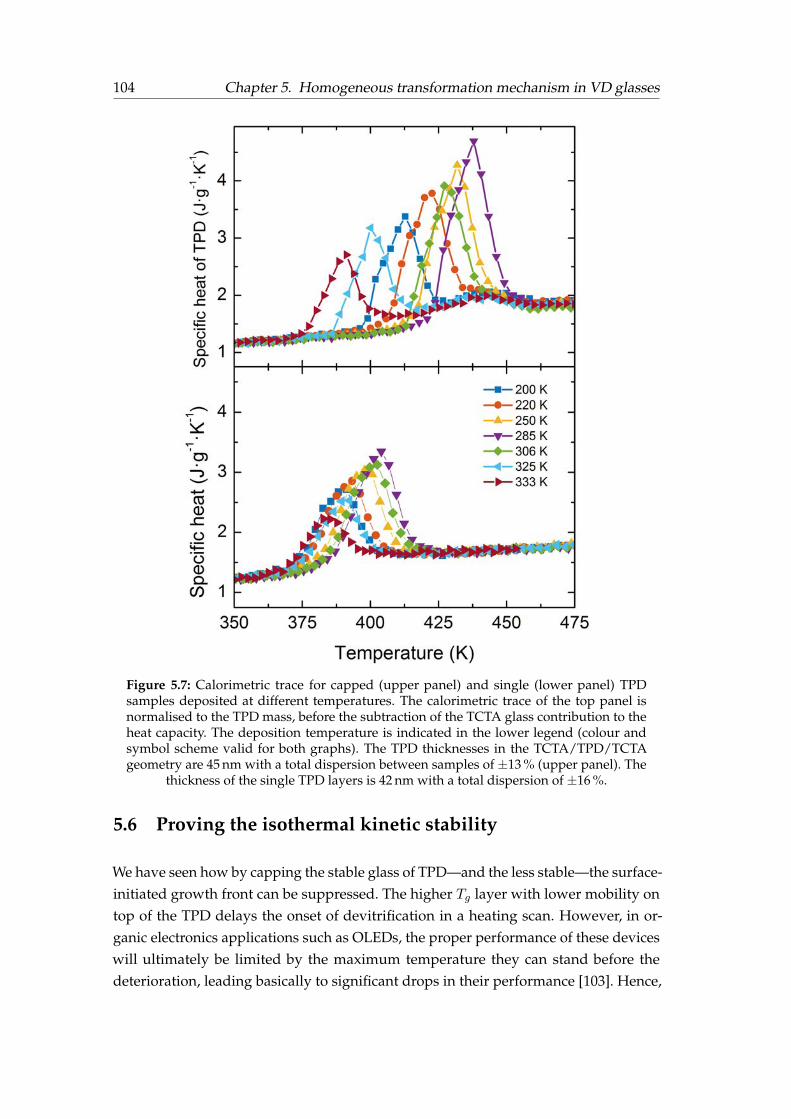
104 Chapter 5. Homogeneous transformation mechanism in VD glasses
Figure 5.7: Calorimetric trace for capped (upper panel) and single (lower panel) TPDsamples deposited at different temperatures. The calorimetric trace of the top panel isnormalised to the TPD mass, before the subtraction of the TCTA glass contribution to theheat capacity. The deposition temperature is indicated in the lower legend (colour andsymbol scheme valid for both graphs). The TPD thicknesses in the TCTA/TPD/TCTAgeometry are 45 nm with a total dispersion between samples of ±13 % (upper panel). The
thickness of the single TPD layers is 42 nm with a total dispersion of ±16 %.
5.6 Proving the isothermal kinetic stability
We have seen how by capping the stable glass of TPD—and the less stable—the surface-initiated growth front can be suppressed. The higher Tg layer with lower mobility ontop of the TPD delays the onset of devitrification in a heating scan. However, in or-ganic electronics applications such as OLEDs, the proper performance of these deviceswill ultimately be limited by the maximum temperature they can stand before thedeterioration, leading basically to significant drops in their performance [103]. Hence,
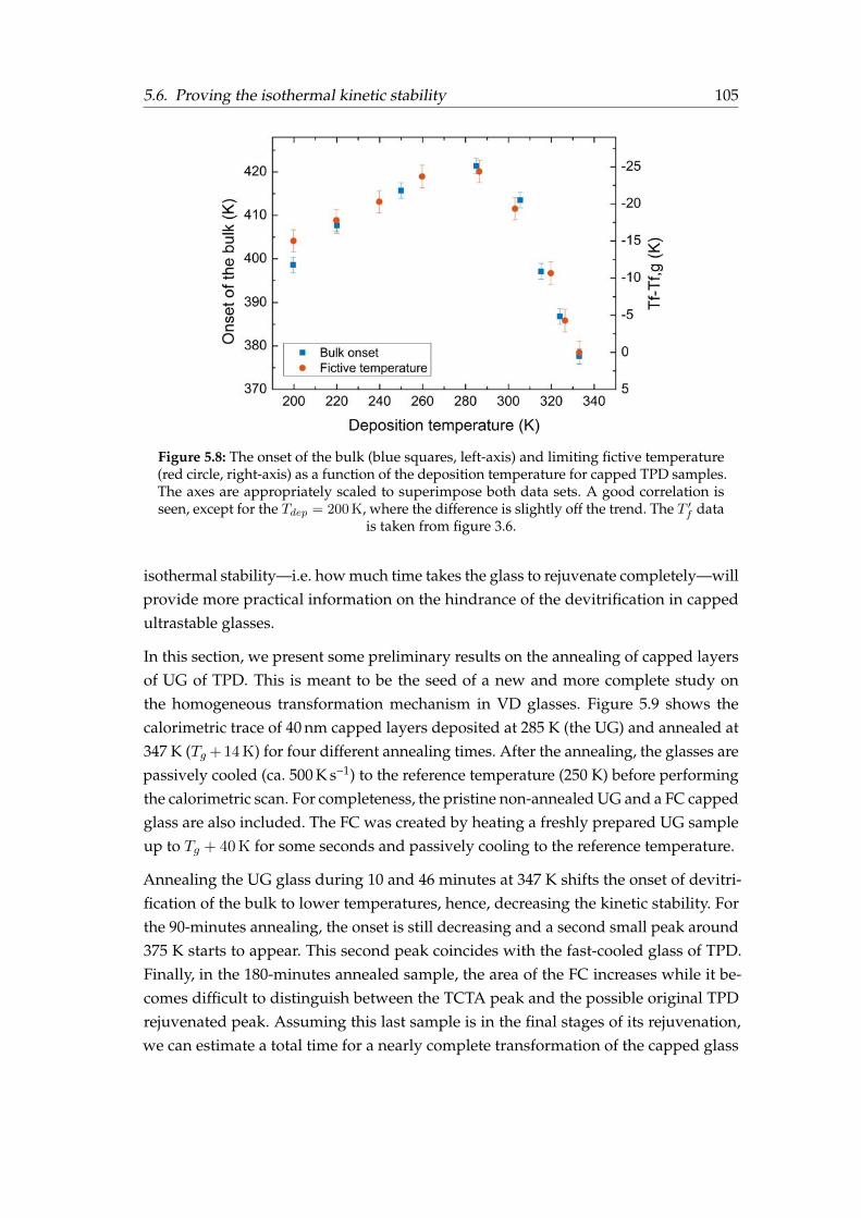
5.6. Proving the isothermal kinetic stability 105
Figure 5.8: The onset of the bulk (blue squares, left-axis) and limiting fictive temperature(red circle, right-axis) as a function of the deposition temperature for capped TPD samples.The axes are appropriately scaled to superimpose both data sets. A good correlation isseen, except for the Tdep = 200 K, where the difference is slightly off the trend. The T ′f data
is taken from figure 3.6.
isothermal stability—i.e. how much time takes the glass to rejuvenate completely—willprovide more practical information on the hindrance of the devitrification in cappedultrastable glasses.
In this section, we present some preliminary results on the annealing of capped layersof UG of TPD. This is meant to be the seed of a new and more complete study onthe homogeneous transformation mechanism in VD glasses. Figure 5.9 shows thecalorimetric trace of 40 nm capped layers deposited at 285 K (the UG) and annealed at347 K (Tg + 14 K) for four different annealing times. After the annealing, the glasses arepassively cooled (ca. 500 K s−1) to the reference temperature (250 K) before performingthe calorimetric scan. For completeness, the pristine non-annealed UG and a FC cappedglass are also included. The FC was created by heating a freshly prepared UG sampleup to Tg + 40 K for some seconds and passively cooling to the reference temperature.
Annealing the UG glass during 10 and 46 minutes at 347 K shifts the onset of devitri-fication of the bulk to lower temperatures, hence, decreasing the kinetic stability. Forthe 90-minutes annealing, the onset is still decreasing and a second small peak around375 K starts to appear. This second peak coincides with the fast-cooled glass of TPD.Finally, in the 180-minutes annealed sample, the area of the FC increases while it be-comes difficult to distinguish between the TCTA peak and the possible original TPDrejuvenated peak. Assuming this last sample is in the final stages of its rejuvenation,we can estimate a total time for a nearly complete transformation of the capped glass

106 Chapter 5. Homogeneous transformation mechanism in VD glasses
Figure 5.9: Capped ultrastable glasses of TPD annealed for different times at 347 K (Tg +14 K). The legend indicates the thickness of the TPD layer together with the annealing time.FC stands for the fast-cooled glass, obtained after an already scanned sample. The black
line corresponds to the specific heat of the TPD glass.
somewhere between 5400 s and 10 800 s. This is only meant to be a first approxima-tion. A more thorough study with more annealing times, annealing temperatures andthicknesses must but carried out to fully characterise the isothermal rejuvenation.
To compare the time that would need a single sample of ultrastable TPD glass to trans-form into the liquid completely, we must use the growth front velocity at Tg + 14 K. Wedo not have access to this temperature regime with the fast-scanning nanocalorimetrytechnique. Walters et al. [40] use ellipsometry and an annealing protocol to provide thetransformation front velocities of TPD glasses up to Tg + 15 K. At 347 K, they found avelocity of around 0.2 nm s−1 for the surface initiated front. Hence, a non-capped TPDsample of 40 nm would take of the order of 200 s to fully transform into the supercooledliquid via this heterogeneous mechanism. We can estimate, therefore, an increase in theisothermal kinetic stability of a factor 25-50, in time units, for a 40 nm stable sample ofTPD. These results are consistent with the data obtained by Sepúlveda et al. [88], wherethey showed how the transformation front of IMC ultrastable glasses was effectivelysuppressed by capping it with a higher Tg material, TNB in that case. They demon-strated how the kinetic stability of a capped glass is substantially enhanced, with theinterface TNB/IMC completely arrested. However, their glass eventually transformedat the interfaces between the stable glasses of indomethacin and the partially deuter-ated indomethacin they used to follow the transformation with SIMS. They argue thatthe kinetic stability might be further enhanced up to a factor of 50 for a 20 nm stableIMC glass without these artificial interfaces used for their measurements, as we are

5.7. Summary 107
showing here.
We have discussed the enhancement of the isothermal stability in terms of the rejuve-nation of the primary peak, following its shift to lower temperatures with time. Theshift of the whole primary peak is indicative of rejuvenation that is taking place co-operatively throughout the entire glass. However, the gradual appearance over timeof the second peak corresponding to the FC glass is indicative of two differentiatedregions. A first one, where a fraction of the glass is homogeneously rejuvenating anda second one that has completely transformed into the supercooled liquid. The latterregion yields, after the fast cooling to the low-temperature transition, the first devitri-fication peak. Having two distinct regions during the annealing protocol is consistentwith the thermodynamic picture where the transformation into the SCL—or melting—occurs via a ‘nucleation and growth’ from the higher mobility regions (liquid) to thelower mobility regions (glass), as conceived by random first order transition theory[17]. However, a note of caution is due here, as having these two distinct regions is alsocompatible with a slower growth front starting at one or both interfaces with TCTAwhich would indicate that the surface mobility is not completely suppressed by theTCTA but highly reduced instead. In fact, this double-peak feature was also observedby Sepúlveda et. al [107] in ultrastable glasses of toluene. However, in that case it wasclearly a front mechanism since they used non-capped films. Further experiments areneeded to explore these possibilities.
5.7 Summary
We have taken a step forward towards enhancing our understanding of the transfor-mation mechanisms of stable glasses by gaining access to the bulk devitrification intothe SCL. By capping the stable glasses of TPD with a higher Tg material we have ef-fectively eliminated the growth front. Using four different multilayer configurations,we have inferred that our single samples of TPD transform through a surface-initiatedfront, which contrasts with the substrate-initiated front found by other authors. Wehave seen how the onset of the devitrification can be delayed up to 40 K by cappingthe free surface of an ultrastable glass, while without capping, this delay was limitedto ≈20 K and thickness-dependent due to the appearance of a transformation front.We have found an excellent correlation between the onset of the bulk and the fictivetemperature for glasses deposited in the 0.6-1.0Tg range. These results provide furthersupport to the kinetic facilitation picture in which these highly packed glasses starttransforming where the mobility is higher.
In a typical OLED device, the active organic layers are capped either by the electrodesor by another organic layer, so it is of vital importance to understand the effect ofcapping on the stability of a glass. We have shown here how the isothermal stability

108 Chapter 5. Homogeneous transformation mechanism in VD glasses
can be enhanced by a 25 to 50 factor if the glass is capped with a higher Tg glass-former. In that sense, this reinforces the idea of employing stable glasses to designorganic electronic devices—OLEDs, for instance—with enhanced temperature stabilityand operational lifetime. However, this last statement remains yet to be thoroughlyaddressed.

Chapter 6
Thermal conductivity onvapour-deposited glasses
6.1 Introduction
In Chapter 1, we have briefly detailed how organic—and inorganic—glasses are essen-tial for a broad range of scientific and technological processes [13]. Particularly, theirapplication into organic semiconductors stands out as a suitable candidate for a newgeneration of electronics due to their inherent flexibility, potential low fabrication costand large area fabrication [7, 108]. Their utilisation in organic electronics applicationsranges from organic light-emitting devices [108] (OLEDs), organic field-effect tran-sistors [109], organic solar cells [110] or even thermoelectric generators[111]. Amongthe different routes for preparing the active layers of these devices, physical vapourdeposition stands out as a prominent technique for small molecule organic semicon-ductors [7], which proves also a suitable tool to tailor the properties of the evaporatedamorphous layers. We have already seen how properties such as thermodynamic andkinetic stability [10, 29, 45, 112] or higher densities [39, 40, 44, 46] can be effectivelyenhanced on different organic molecules when evaporating at substrate temperaturesof 0.80-0.90Tg. Moreover, the orientation of the molecules also depends on the depo-sition temperature as seen with birefringence [39] and dichroism [45] measurements.However, to date, only a few studies are addressing the thermal conductivity of glassythin films of small organic semiconductors molecules [113, 114], and none of them havefocused on the role that molecular anisotropy or other glass features such as densityvariations, play on this property. However, several studies are addressing the thermalconductivity in organic semiconductor crystals [115–117].
Most of the works in organic electronics are focused on the electronic transport prop-erties since this is a key parameter for the employment of these materials in optoelec-tronic devices. Nonetheless, thermal transport and thermal management in organicdevices are becoming increasingly important, in particular for scaled-up large areaapplications and for the integration of these devices in complex arrays and systems.

110 Chapter 6. Thermal conductivity on vapour-deposited glasses
Generally, the thermal conductivity in amorphous organic semiconductors is muchlower than in traditional inorganic semiconductors [113, 118, 119], with typical valuesbelow 1 W m−1 K−1. For the sake of comparison, silicon substrates used in microelec-tronics applications have a thermal conductivity of 150 W m−1 K−1and stainless steelof 16 W m−1 K−1 [120]. For instance, during its normal operation, OLED devices sufferthermal stress and degradation [121]. Luminance and lifetime also decrease when op-erated at high temperatures [103]. Localized Joule heating effects can highly reducebrightness homogeneity and it can be worsened as temperature increases with opera-tion time [122]. Chung et al. showed how the lifetime of an OLED could be effectivelyenhanced by decreasing the peak temperature with efficient heat dissipation using, intheir case, different substrates [123]. Although the heat capacities and the conductiv-ity of active layers from these devices are rather small, evaluating the details of theheat generation and dissipation are required to fully understand the impact on theirperformance. Furthermore, recent studies are starting to pay attention also to organicsemiconductors due to their potential for thermoelectric applications [124, 125]. Theirsemiconductor nature and the low thermal conductivities make them potential candi-dates to improve the thermoelectric figure-of-merit ZT. We note most of the previousstudies in this direction have been reported for polymer-based devices and very fewon small molecule organic semiconductors. Therefore, either for thermal managementof organic devices or for thermoelectric applications, a key parameter that must beknown is the thermal conductivity. Even more interesting than assessing its value, isthe possibility of modifying it. Wang et al. reported the feasibility of tailoring the ther-mal conductivity of a novel organic semiconductor used in transistor devices with Agnanoparticles [126], for which they measured the out-of-plane thermal conductivity.
The main difficulty towards a comprehensive analysis of the thermal conductivityarises from the lack of appropriate techniques to measure the in-plane thermal trans-port properties in thin films. Previous measurements on polymers or polymer nanofiberswere conducted on suspended structures [127, 128] which directly provide the in-planethermal conductance. This methodology, frequently used for inorganic nanowires oflow thermal conductance, requires lengthy or sophisticated approaches to preciselyplace the sample bridging the heater/sensor platforms and it is not directly applicableto the kind of organic thin films of interest in this work. We have recently shown that amodification of the 3ω–Völklein technique [83, 84] can be used to monitor in real-timethe growth of organic layers and to measure their in-plane thermal conductance (k‖)[129]. The high sensitivity of the technique and its versatility makes it an ideal tool toexplore the in-plane thermal transport characteristics of organic thin films.
In this chapter, we use the modification of the 3ω–Völklein technique explained in Sec-tion 2.4 to measure, in situ, the thermal conductance of films of organic glass-formers

6.2. Monitoring thermal conductivity during the film growth 111
during and after its growth. We first use the high sensitivity of the technique to moni-tor in real-time the first stages of thin film growth of the hole transport materials TPDand α-NPD. The influence of the deposition temperature on the percolation thresholdis also addressed. The in-plane thermal conductivity data is complemented with out-of-plane thermal conductivity (k⊥) measurements using the standard 3ω technique,briefly described in Section 2.4.5. We investigate the impact that the deposition temper-ature impinges on the thermal conductivity of TPD and α-NPD films. The depositiontemperature has a direct bearing on density, thermal and kinetic stability and molec-ular orientation, among other properties. Hence, we discuss the effect that all theseproperties have in the measured thermal conductivities.
6.2 Monitoring thermal conductivity during the film growth
Having the 3ω–Völklein sensors inside the UHV evaporation chamber allows not onlyto measure in situ the thermal conductivity of the deposited layer but also to monitorits evolution during the growth of the layer. To obtain the V3w amplitude, we use atime window equal to 3 current periods, which is translated into a time resolution of3 s for a current waveform of 1 Hz during the growth of the layer. To achieve sub-nmresolution during the growth of the layers, we must use very low deposition rates. Westart by monitoring the thermal conductance of TPD layers while growing them at arate of 0.02 nm s−1 for two different Tdep, (267± 2) K and (304± 2) K . The temperatureuncertainty is due to the oscillation produced by the current wave. We also measure thegrowth of an α-NPD layer deposited at (296± 1) K at a rate of 0.015 nm s−1. In this case,we use the same current wave amplitude but a frequency of 0.5 Hz, which is translatedin a time window of 6 s for each measurement.
Figures 6.1a and 6.1b show the evolution of the conductance (G) versus thickness forthe two TPD layers deposited at 267 K (0.80Tg) and 304 K (0.91Tg), respectively. In theinset of Figure 6.1a, the electrical conductance is represented versus the thickness ofa TPD layer during its growth on top of a nitride membrane. Figure 6.2a shows thegrowth of α-NPD film deposited at 297 K (0.81Tg) whereas Figure 6.2b shows againan α-NPD film grown at the same temperature but deposited on top of a pre-existingcontinuous α-NPD layer.
We have identified four distinct regions during the growth of the OSG layers for thefirst three samples. Region I is characterised by an exponential drop of the conductanceof the membrane in the first three cases. In region II, the decrease is slowed down toa minimum until it reaches region III, where the G starts to increase monotonically.Between region III and IV, there is a change into a linear regime of G versus thickness.As explained below, we can identify these regions with the growth modes of a filmon a substrate: the first initial drop in region I corresponds to nucleation and island

112 Chapter 6. Thermal conductivity on vapour-deposited glasses
(a) Layer grown at Tdep = (267± 2) K,0.80Tg
(b) Layer grown at Tdep = (304± 2) K,0.91Tg .
Figure 6.1: Thermal conductance versus film thickness during the deposition of a TPDlayer. The layers are deposited at 0.02 nm s−1. The vertical lines separate the differentgrowth regions. Region I, between zero nanometers and the first line, correspond to nucle-ation and isolated island growth; region II to island growth and subsequent coalescence;region III marks the percolation across the surface until region IV is reached, where the ver-tical growth of a continuous layer starts. The inset of the Figure 6.1a shows the evolution
of the electrical conductance during the growth of an equivalent TPD film.
growth, in region II the islands grow until they start to coalesce; region III marks theonset of the percolation until the full surface is covered at the onset of region IV, wherethe film starts the vertical and continuous growth. Amorphous organic layers growfollowing a 3D Volmer-Weber mechanism with isolated islands in the early growthstages on top of a silicon nitride substrate. This is further supported by Figure 6.3which shows the presence of isolated islands for a 2.6 nm (nominal thickness) film ofTPD grown at 0.80Tg (AFM image) whereas the 14.3 nm film is already continuous(SEM image). The morphological study of the vapour deposited samples was carriedout ex situ and in different evaporation runs. This adds some uncertainty to the onsetsof the different growth modes in our samples. Moreover, Zhang et al. [130] showed howsurface diffusion in TPD was greatly enhanced compared to the bulk, using preciselythe morphological changes in their surfaces to infer its value, even at room temperature.This prevents us from providing a thorough analysis of the topology evolution of ourthin layers using either ex situ AFM or SEM.
6.2.1 Interpretation of the growth regions
The first fast initial drop in thermal conductance seen in region I of Figures 6.1a, 6.1band 6.2a can be attributed to the nucleation and formation of the first islands on the topof the nitride membrane. To interpret the evolution of the thermal conductance withthe organic film thickness we must first comment on the intrinsic thermal conductivityof the nitride membrane. The disordered nature of the membrane is consistent with the
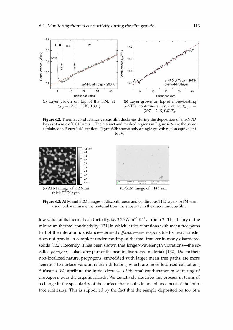
6.2. Monitoring thermal conductivity during the film growth 113
(a) Layer grown on top of the SiNx atTdep = (296± 1) K, 0.80Tg
(b) Layer grown on top of a pre-existingα-NPD continuous layer at at Tdep =
(297± 2) K, 0.81Tg .
Figure 6.2: Thermal conductance versus film thickness during the deposition of a α-NPDlayers at a rate of 0.015 nm s−1. The distinct and marked regions in Figure 6.2a are the sameexplained in Figure’s 6.1 caption. Figure 6.2b shows only a single growth region equivalent
to IV.
(a) AFM image of a 2.6 nmthick TPD layer.
(b) SEM image of a 14.3 nm
Figure 6.3: AFM and SEM images of discontinuous and continuous TPD layers. AFM wasused to discriminate the material from the substrate in the discontinuous film.
low value of its thermal conductivity, i.e. 2.25 W m−1 K−1 at room T . The theory of theminimum thermal conductivity [131] in which lattice vibrations with mean free pathshalf of the interatomic distance—termed diffusons—are responsible for heat transferdoes not provide a complete understanding of thermal transfer in many disorderedsolids [132]. Recently, it has been shown that longer-wavelength vibrations—the so-called propagons—also carry part of the heat in disordered materials [132]. Due to theirnon-localized nature, propagons, embedded with larger mean free paths, are moresensitive to surface variations than diffusons, which are more localised excitations,diffusons. We attribute the initial decrease of thermal conductance to scattering ofpropagons with the organic islands. We tentatively describe this process in terms ofa change in the specularity of the surface that results in an enhancement of the inter-face scattering. This is supported by the fact that the sample deposited on top of a
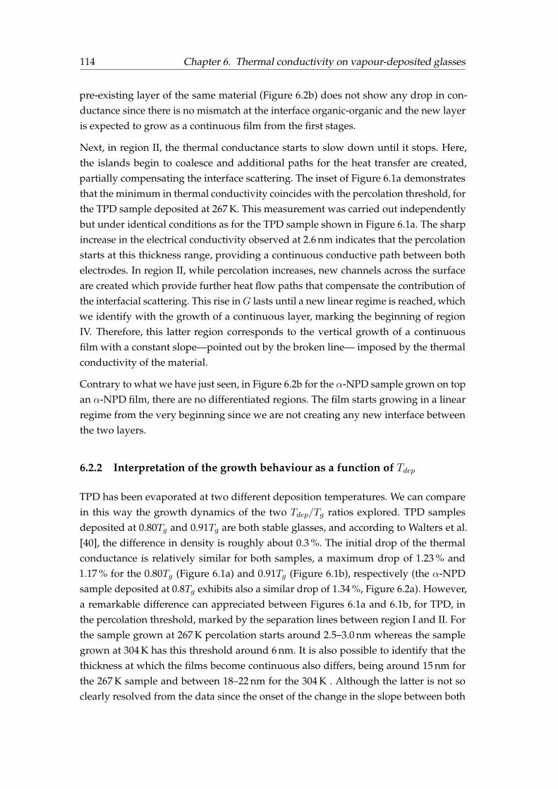
114 Chapter 6. Thermal conductivity on vapour-deposited glasses
pre-existing layer of the same material (Figure 6.2b) does not show any drop in con-ductance since there is no mismatch at the interface organic-organic and the new layeris expected to grow as a continuous film from the first stages.
Next, in region II, the thermal conductance starts to slow down until it stops. Here,the islands begin to coalesce and additional paths for the heat transfer are created,partially compensating the interface scattering. The inset of Figure 6.1a demonstratesthat the minimum in thermal conductivity coincides with the percolation threshold, forthe TPD sample deposited at 267 K. This measurement was carried out independentlybut under identical conditions as for the TPD sample shown in Figure 6.1a. The sharpincrease in the electrical conductivity observed at 2.6 nm indicates that the percolationstarts at this thickness range, providing a continuous conductive path between bothelectrodes. In region II, while percolation increases, new channels across the surfaceare created which provide further heat flow paths that compensate the contribution ofthe interfacial scattering. This rise inG lasts until a new linear regime is reached, whichwe identify with the growth of a continuous layer, marking the beginning of regionIV. Therefore, this latter region corresponds to the vertical growth of a continuousfilm with a constant slope—pointed out by the broken line— imposed by the thermalconductivity of the material.
Contrary to what we have just seen, in Figure 6.2b for the α-NPD sample grown on topan α-NPD film, there are no differentiated regions. The film starts growing in a linearregime from the very beginning since we are not creating any new interface betweenthe two layers.
6.2.2 Interpretation of the growth behaviour as a function of Tdep
TPD has been evaporated at two different deposition temperatures. We can comparein this way the growth dynamics of the two Tdep/Tg ratios explored. TPD samplesdeposited at 0.80Tg and 0.91Tg are both stable glasses, and according to Walters et al.[40], the difference in density is roughly about 0.3 %. The initial drop of the thermalconductance is relatively similar for both samples, a maximum drop of 1.23 % and1.17 % for the 0.80Tg (Figure 6.1a) and 0.91Tg (Figure 6.1b), respectively (the α-NPDsample deposited at 0.8Tg exhibits also a similar drop of 1.34 %, Figure 6.2a). However,a remarkable difference can appreciated between Figures 6.1a and 6.1b, for TPD, inthe percolation threshold, marked by the separation lines between region I and II. Forthe sample grown at 267 K percolation starts around 2.5–3.0 nm whereas the samplegrown at 304 K has this threshold around 6 nm. It is also possible to identify that thethickness at which the films become continuous also differs, being around 15 nm forthe 267 K sample and between 18–22 nm for the 304 K . Although the latter is not soclearly resolved from the data since the onset of the change in the slope between both

6.3. Thermal conductivity dependence on deposition temperature 115
regions is subtle. Notwithstanding, the different growth dynamics is unmistakablyidentified by the different behaviour in region III. In the sample grown at 267 K, thethermal conductance in the percolation region increases faster than the vertical growthfrom region IV. In contrast, the sample deposited at 304 K exhibits a smaller slope inregion III.
We can now rationalise these findings qualitatively in terms of surface diffusivity. As-suming that surface tension changes only slightly in this temperature range, variationsin surface mobility with substrate temperature could be at the origin of the observedbehaviour. According to Zhang and co-workers [130] surface mobility in TPD is ofArrhenius-type with values of Ds = 7× 10⁻¹⁸ m2 s−1 at 304 K and 8× 10⁻¹⁹ m2 s−1 at296 K. Extrapolating to 267 K leads to Ds = 4× 10⁻²³ m2 s−1. With those values andusing x ≈ (4Dt)1/2 as the mean distance molecules diffuse during time t, it is possi-ble to roughly infer if island formation is driven by diffusion-limited aggregation orby attachment-limited aggregation mechanisms. As growth rate was 0.02 nm s−1 theresidence time of surface molecules before being buried by new molecules impingingfrom the vapour is of the order of 25 s for a 1 nm layer. Therefore, at Tdep = 304 K, x ≈26 nm while at Tdep = 267 K , x ≈ 0.06 nm. Within this assumption, the layer at 267 Kwill be composed of many, but small, islands, while growth at 304 K will result in less,but larger islands. This is compatible with the results of Figure 6.2a which shows thatfilms grown at 267 K achieve the onset of percolation and a continuous film at smallerthicknesses compared to the sample grown at higher T . Although we do not have twotemperatures for the sake of comparison for the α-NPD, the sample grown at 0.80Tgbehaves similarly to the equivalent TPD sample, i.e. drop of thermal conductance uponisland formation, percolation threshold thickness at around 3.5 nm and continuous filmat 13 nm. Our threshold for continuous films is in agreement with recent work from[130]. In their work, they obtained uniform layers at thicknesses above 20 nm, althoughtheir films were deposited at a higher temperature of 330 K (0.99Tg). A complete analy-sis of these growth mechanisms is out of the scope of this work, but it seems clear thatthe 3ω–Völklein technique opens a new avenue to unravel the physics of film growthof vapour-deposited glasses.
6.3 Thermal conductivity dependence on deposition tempera-ture
We focus now our attention on the dependence of the thermal conductivities for con-tinuous films of TPD and α-NPD over a wide range of deposition temperatures, from220 K to 333 K and 368 K, respectively. For these measurements, we do not require thelow deposition rates we needed to follow the early stages of the growing films. Hence,

116 Chapter 6. Thermal conductivity on vapour-deposited glasses
we use faster rates of (0.21± 0.02) nm s−1 and (0.10± 0.02) nm s−1 for TPD and α-NPD,respectively—similar to the rates used for the heat capacity characterisation.
Our aim is to compare the thermal conductivity of samples grown at different temper-atures but measured at equal conditions. We start measuring the conductance of TPDfilms using two different approaches at each deposition temperature. In the first one,we carry out single conductance measurements on 340 nm thick layers evaporated di-rectly on the clean surface of the membrane. As explained in Section 2.4.3, the in-planeconductivity k‖ can be obtained from the slope of the linear regime (region IV) usingequation 2.24. Although the dependence of k with temperature is weak in organicamorphous systems [74], we must compare values measured at the same temperature—precluding us to use the slope of equation 2.24 to extract the conductivity. So, aftereach deposition at a certain Tdep, the sample is set back to a reference temperature,Tref , where all the conductivity measurements are performed. The conductance atTref is obtained from the difference in the measured conductance before, and after thedeposition of the film, that is
Gfilm = Gtotal −GSiNx (6.1)
Once the thermal conductance is measured, we can make use of equation 2.20 to get thethermal conductivity considering the thickness of the film and length of the sensor’sstrip. The amplitude of the current waveform injected to the sensor is chosen accord-ingly to produce a ∆T = 4 K at a frequency of 1 Hz. While the reference temperatureis set to 295 K, the effective temperature is (297± 1) K, due to the thermal oscillationsproduced by the current wave across the sensing area. After each deposition, the sen-sor is cleaned outside the UHV chamber using acetone and ethanol, and preparedfor the subsequent evaporation. The thermal conductivity values obtained using thisprocedure are shown in Figure 6.5 (labelled as single-layer) as a function of Tdep. Thismethod is time-consuming as it requires opening and closing the UHV chamber foreach measurement. Moreover, the sensor must be manipulated between measurementsfor the manual cleaning and the wiring to the socket with the consequent membraneweakening or possible structural damage.
In the second approach, the thermal conductance of samples prepared at several de-position temperatures is measured in a single run at a reference temperature of 296K. Without breaking the vacuum, 150 nm thick layers are grown on top of each otherat different Tdep while the conductance measurements are performed in-between de-positions. Figure 6.4 represents a scheme of the followed protocol. The depositiontemperature in two consecutive samples is deliberately alternated between temper-atures above and below Tref . In such a way, the effects of conceivable instrumentaldrifts when evaluating k are randomised. For instance, we start measuring the con-ductance of the bare SiNx membrane to get the initial conductance at the reference

6.3. Thermal conductivity dependence on deposition temperature 117
Figure 6.4: Temperature scheme followed (blue-line) to measure the thermal conductanceof multiple layers evaporated at different substrate temperatures. The conductance ofeach layer (red-line) is obtained as the differential increment between two consecutive
evaporations, always at a reference temperature of 295 K, as indicated in equation 6.2.
temperature. Then, we evaporate a 150 nm layer at this same temperature, and theconductance starts growing until the layer is finished. The conductance of the layeris obtained again as the differential measurement, following the expression 6.1. Wethen increase the substrate temperature and so does the conductance because of thetemperature. We evaporate a layer of the same thickness at this new temperature, andG increases linearly. Once deposited, the temperature is set back to Tref , and the newG is measured again. Therefore, the layer conductance is obtained as the differentialincrement before and after each deposition, following the straightforward expression:
Gfilm,i = Gtotal,i −Gtotal,i−1 (6.2)
where i corresponds to each step.
The scheme is then repeated for another set of deposition temperatures. For this typeof measurement, we use a frequency of 0.5 Hz for the current waveform, instead ofthe 1 Hz used in the previous approach. As explained in Section 2.4.3, lowering thefrequency increases the accuracy of the measurements as well as it decreases the G2ω
dependence on other properties of the sample. This allows us to measure thicker sam-ples without compromising the accuracy of the conductance. For instance, if we goback to Figure 2.14, we can see how for a frequency of 0.5 Hz, the G2ω is less than1 % away from the real conductance. In this second approach, the amplitude of thecurrent wave is also reduced, producing, in this case, a ∆T = 2.25 K. Finally, when

118 Chapter 6. Thermal conductivity on vapour-deposited glasses
Figure 6.5: Measured thermal conductivity of TPD glasses as a function of Tdep and mea-sured at (296± 1) K. The two different procedures are labelled as single-layer measurementsand multilayer measurements. Hence, each blue-square value is obtained from indepen-dent evaporations of 340 nm thick layers, cleaning the sensor after each sample deposition.Circle and triangle points are obtained following the continuous method, in which a mul-tilayer is deposited, and the conductivity measured differentially between 150 nm thicklayers. Three independent devices (D1, D2, D3) have been used for the determination ofG. The error bars are calculated from uncertainty in the thickness determination from
profilometry.
using this approach, we are assuming that the glass layers are not affected by a possi-ble rejuvenation or ageing when depositing the different layers. As long as the Tdep iskept below Tg and the deposition times short compared to the vast timescales requiredfor rejuvenation, this effect is hindered. The results obtained using this procedure areshown in Figure 6.5, labelled as multilayer, together with the results obtained using theother approach. In all cases, the use of different devices is labelled as sensor Di (wherei stands for the device number).
From Figure 6.5 it is clearly seen that the two approaches are in reasonable agreement.As commented in Section 2.4, the sensitivity of this technique is remarkably high, about∆G/G ' 10−3 in conductance. However, the final accuracy of the thermal conductiv-ity is not limited by the conductance measurement itself but from the uncertainty inthe amount of mass sensed. The uncertainty in the initial calibration using profilom-etry is of ±2 nm, represented by the error bars in Figure 6.5 using the correspondingerror propagation. However, other factors such as the reproducibility in the readingof the QCM or the use of different devices might contribute to the small dispersion.Using 95 % confidence interval for the standard error for Tdep with more than onepoint we can estimate an upper limit of the statistical error in thermal conductivity of±0.004 W m−1 K−1.
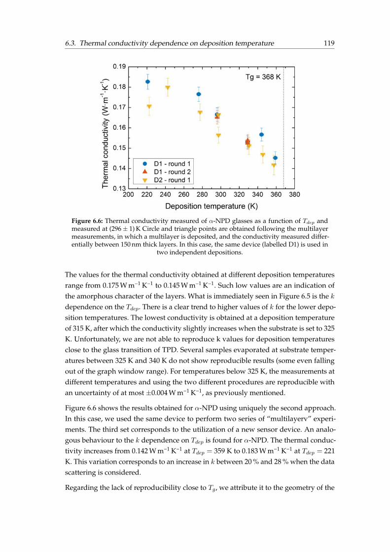
6.3. Thermal conductivity dependence on deposition temperature 119
Figure 6.6: Thermal conductivity measured of α-NPD glasses as a function of Tdep andmeasured at (296± 1) K Circle and triangle points are obtained following the multilayermeasurements, in which a multilayer is deposited, and the conductivity measured differ-entially between 150 nm thick layers. In this case, the same device (labelled D1) is used in
two independent depositions.
The values for the thermal conductivity obtained at different deposition temperaturesrange from 0.175 W m−1 K−1 to 0.145 W m−1 K−1. Such low values are an indication ofthe amorphous character of the layers. What is immediately seen in Figure 6.5 is the kdependence on the Tdep. There is a clear trend to higher values of k for the lower depo-sition temperatures. The lowest conductivity is obtained at a deposition temperatureof 315 K, after which the conductivity slightly increases when the substrate is set to 325K. Unfortunately, we are not able to reproduce k values for deposition temperaturesclose to the glass transition of TPD. Several samples evaporated at substrate temper-atures between 325 K and 340 K do not show reproducible results (some even fallingout of the graph window range). For temperatures below 325 K, the measurements atdifferent temperatures and using the two different procedures are reproducible withan uncertainty of at most ±0.004 W m−1 K−1, as previously mentioned.
Figure 6.6 shows the results obtained for α-NPD using uniquely the second approach.In this case, we used the same device to perform two series of “multilayerv” experi-ments. The third set corresponds to the utilization of a new sensor device. An analo-gous behaviour to the k dependence on Tdep is found for α-NPD. The thermal conduc-tivity increases from 0.142 W m−1 K−1 at Tdep = 359 K to 0.183 W m−1 K−1 at Tdep = 221K. This variation corresponds to an increase in k between 20 % and 28 % when the datascattering is considered.
Regarding the lack of reproducibility close to Tg, we attribute it to the geometry of the
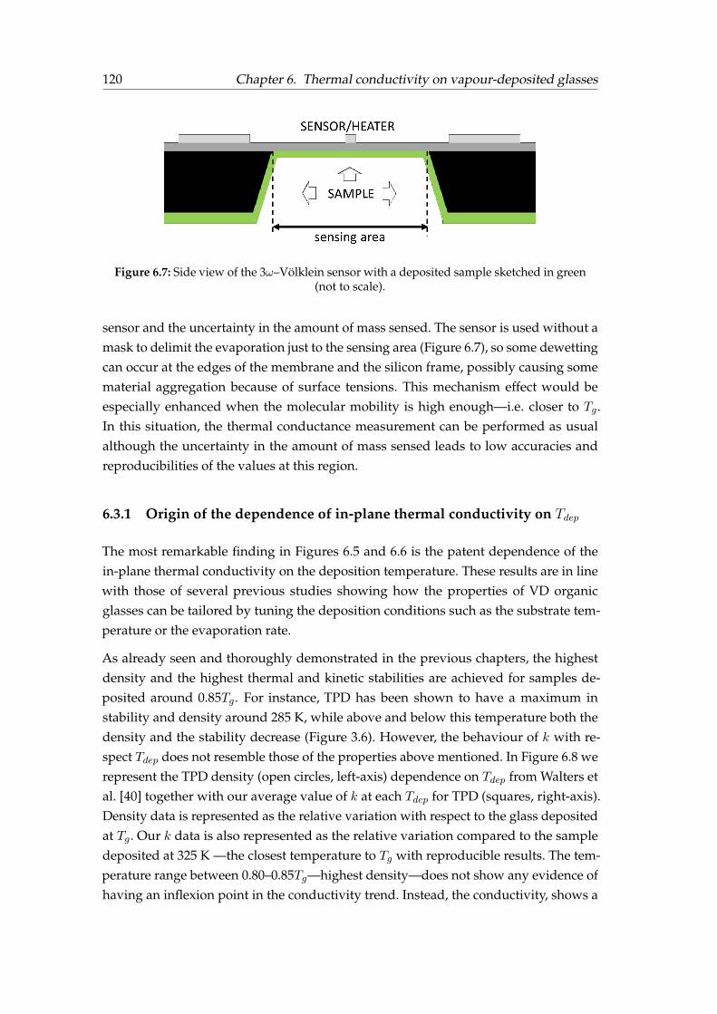
120 Chapter 6. Thermal conductivity on vapour-deposited glasses
Figure 6.7: Side view of the 3ω–Völklein sensor with a deposited sample sketched in green(not to scale).
sensor and the uncertainty in the amount of mass sensed. The sensor is used without amask to delimit the evaporation just to the sensing area (Figure 6.7), so some dewettingcan occur at the edges of the membrane and the silicon frame, possibly causing somematerial aggregation because of surface tensions. This mechanism effect would beespecially enhanced when the molecular mobility is high enough—i.e. closer to Tg.In this situation, the thermal conductance measurement can be performed as usualalthough the uncertainty in the amount of mass sensed leads to low accuracies andreproducibilities of the values at this region.
6.3.1 Origin of the dependence of in-plane thermal conductivity on Tdep
The most remarkable finding in Figures 6.5 and 6.6 is the patent dependence of thein-plane thermal conductivity on the deposition temperature. These results are in linewith those of several previous studies showing how the properties of VD organicglasses can be tailored by tuning the deposition conditions such as the substrate tem-perature or the evaporation rate.
As already seen and thoroughly demonstrated in the previous chapters, the highestdensity and the highest thermal and kinetic stabilities are achieved for samples de-posited around 0.85Tg. For instance, TPD has been shown to have a maximum instability and density around 285 K, while above and below this temperature both thedensity and the stability decrease (Figure 3.6). However, the behaviour of k with re-spect Tdep does not resemble those of the properties above mentioned. In Figure 6.8 werepresent the TPD density (open circles, left-axis) dependence on Tdep from Walters etal. [40] together with our average value of k at each Tdep for TPD (squares, right-axis).Density data is represented as the relative variation with respect to the glass depositedat Tg. Our k data is also represented as the relative variation compared to the sampledeposited at 325 K —the closest temperature to Tg with reproducible results. The tem-perature range between 0.80–0.85Tg—highest density—does not show any evidence ofhaving an inflexion point in the conductivity trend. Instead, the conductivity, shows a
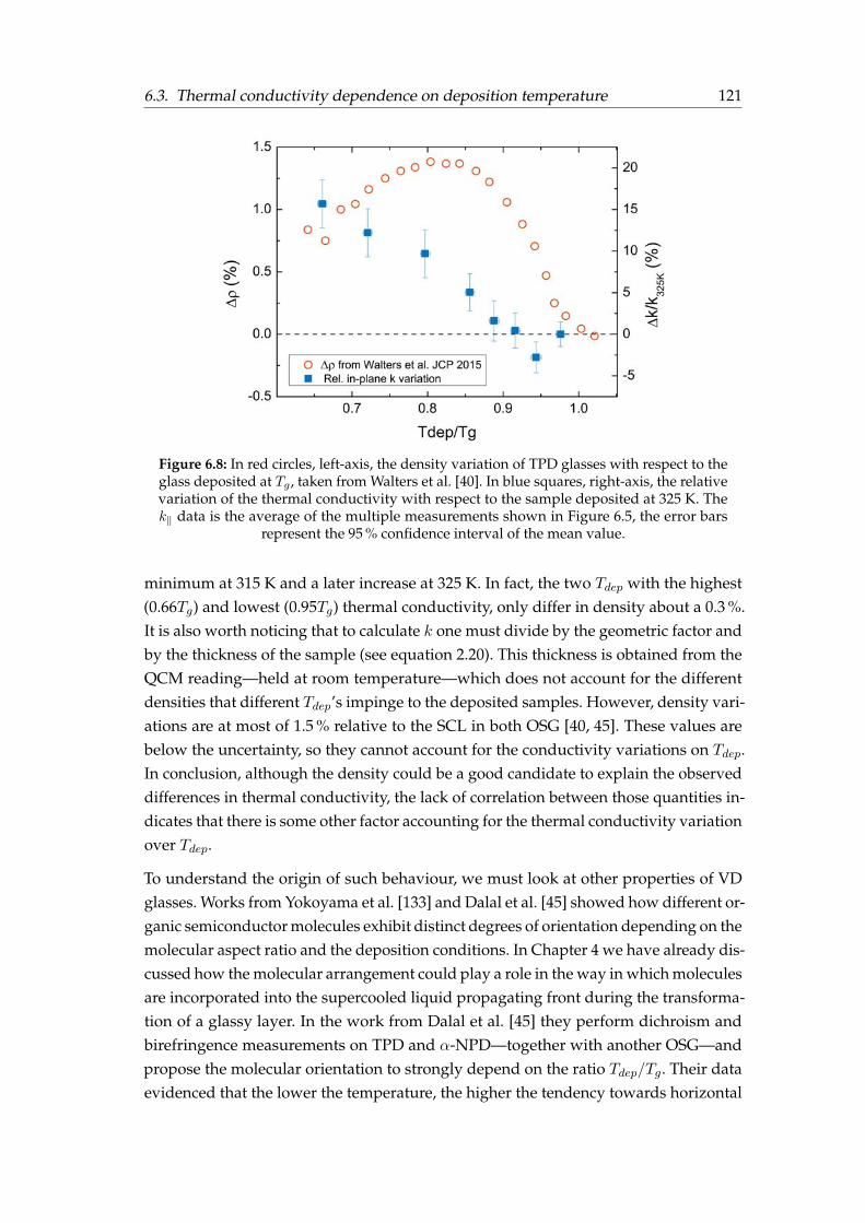
6.3. Thermal conductivity dependence on deposition temperature 121
Figure 6.8: In red circles, left-axis, the density variation of TPD glasses with respect to theglass deposited at Tg , taken from Walters et al. [40]. In blue squares, right-axis, the relativevariation of the thermal conductivity with respect to the sample deposited at 325 K. Thek‖ data is the average of the multiple measurements shown in Figure 6.5, the error bars
represent the 95 % confidence interval of the mean value.
minimum at 315 K and a later increase at 325 K. In fact, the two Tdep with the highest(0.66Tg) and lowest (0.95Tg) thermal conductivity, only differ in density about a 0.3 %.It is also worth noticing that to calculate k one must divide by the geometric factor andby the thickness of the sample (see equation 2.20). This thickness is obtained from theQCM reading—held at room temperature—which does not account for the differentdensities that different Tdep’s impinge to the deposited samples. However, density vari-ations are at most of 1.5 % relative to the SCL in both OSG [40, 45]. These values arebelow the uncertainty, so they cannot account for the conductivity variations on Tdep.In conclusion, although the density could be a good candidate to explain the observeddifferences in thermal conductivity, the lack of correlation between those quantities in-dicates that there is some other factor accounting for the thermal conductivity variationover Tdep.
To understand the origin of such behaviour, we must look at other properties of VDglasses. Works from Yokoyama et al. [133] and Dalal et al. [45] showed how different or-ganic semiconductor molecules exhibit distinct degrees of orientation depending on themolecular aspect ratio and the deposition conditions. In Chapter 4 we have already dis-cussed how the molecular arrangement could play a role in the way in which moleculesare incorporated into the supercooled liquid propagating front during the transforma-tion of a glassy layer. In the work from Dalal et al. [45] they perform dichroism andbirefringence measurements on TPD and α-NPD—together with another OSG—andpropose the molecular orientation to strongly depend on the ratio Tdep/Tg. Their dataevidenced that the lower the temperature, the higher the tendency towards horizontal

122 Chapter 6. Thermal conductivity on vapour-deposited glasses
Figure 6.9: In blue squares, left-axis, the relative variation of the TPD thermal conductivityconcerning the sample deposited at 325 K (notice the inverted y-axis). In red triangles,
right-axis, the order parameter Sz for TPD taken from Dalal et al. [45]
orientation, reaching a plateau at low temperatures. Figure 6.9 shows the relative vari-ation in thermal conductivity (blue squares, left-axis) normalised to the 325 K valueof 0.152 W m−1 K−1—which coincides both with the highest temperature with repro-ducible results and the temperature at which the sample is already isotropic. In theright axis and red triangles, the order parameter Sz from reference [45] is plotted witha common x-axis. The order parameter Sz is a measure of the average orientation ofthe long axis of the molecules relative to the surface normal. A value of −0.5 indicatesall the molecules lying parallel in the plane of the substrate; zero indicates randomorientation and a value of one indicates a perfect vertical alignment. The correlationbetween this parameter and the thermal conductivity variation is remarkably good, asseen in Figure 6.9 for TPD. When the molecules are more horizontally oriented, the in-plane thermal conductivity is higher. From Figure 6.9, it is worth noticing that even thesmall peak at 315 K (0.95Tg)—indicating a slight tendency to vertical orientation—isalso reproduced in the thermal conductivity, showing its lowest value for the in-planeconductivity and proving the high sensitivity of the technique. Figure 6.10 representsthe equivalent representation of Figure 6.9 but for α-NPD this time. Although the datafrom Figure 6.10 show more uncertainty, we see how the same argument is still validalso for this molecule, which reinforces the role that molecular orientation plays in thethermal conductivity.
6.3.2 Out-of-plane thermal conductivity measurements
Our results suggest that heat transport in the parallel direction is favoured whenmolecules have the propensity to lie with the long molecular axis (along with the

6.3. Thermal conductivity dependence on deposition temperature 123
Figure 6.10: In blue squares, left-axis, the relative variation of the α-NPD thermal con-ductivity concerning the sample deposited at 325 K (notice the inverted y-axis). In red
triangles, right-axis, the order parameter Sz for α-NPD taken from Dalal et al. [45]
N-N axis, see Figure 2.5b) parallel to the surface. On the contrary, the resistance toin-plane thermal transport is higher when molecules are isotropically oriented or evenhave a slight tendency to align in the out-of-plane direction. At first glimpse, thisis somewhat surprising given the small size of the molecular unit and the disorderinherent to the glass. To confirm the existence of thermal anisotropy we carried outout-of-plane thermal conductivity (k⊥) measurements with the 3ω technique for thinfilms (see Section 2.4.5 for further details) on two TPD samples: one grown at Tdep =
220 K with the molecules preferentially aligned parallel to the substrate and anotherat Tdep = 304 K with isotropic orientation. As the k⊥ measurement required an ex situpreparation, the sample deposited at Tdep = 304 K (0.91Tg) was chosen as the isotropicrepresentation—instead of sample deposited closer to Tg—because of its higher ther-mal stability. An out-of-plane thermal conductivity of (0.18± 0.02) W m−1 K−1 wasobtained for the anisotropic sample and a value of (0.23± 0.02) W m−1 K−1 for theisotropic one.
The value for the k⊥ for Tdep = 304 K is in agreement with the value found in litera-ture. Kim et al. [113] obtained a value of 0.24 W m−1 K−1 for the out-of-plane thermalconductivity of TPD films deposited at room temperature. Although the room tem-perature value is not specified in their work, it will be presumably close to the 304 Ksample prepared here. However, the absolute values obtained for k‖ and k⊥ (both ourand literature values) are not in agreement. The discrepancy in the accuracy of thevalues is expected to come from the k⊥ measurements. These values are affected bytwo factors that differ from the in-plane measurements. First, in this geometry, there

124 Chapter 6. Thermal conductivity on vapour-deposited glasses
Figure 6.11: Schematics representation showing the relative variation of thermal conduc-tivity (in-plane and out-of-plane) for the anisotropic sample at Tdep = 220 K. For the sake ofcomparison, we have assumed that k⊥ and k‖ are the same in the isotropic sample (Tdep =
304 K) and we have used this values as a reference for the anisotropic sample.
are several interface thermal resistances between the layers which can affect the accu-racy of the values obtained. From the sample measurements, we have the interfaceelectrode/organic and organic/SiNx whereas from the reference measurement there isalso the interface electrode/SiNx. Secondly, the k⊥ is obtained from the approximationof the one-dimensionality of the heat propagation. That propagation holds true as longas the half-width of the strip is much larger than the thickness of the film coveredw >> tfilm. The validity of this approximation for these measurements is commentedin Section 2.4.5. None the less, it is interesting to note that these potential shortcomingsthat limit the accuracy of the absolute value of k⊥ do not affect the relative variationof the 3ω measurements carried out on the two samples grown at a different Tdep. Inboth measurements, the mentioned two factors equally impact the accuracy of the mea-sured thermal conductivity. Therefore, it is safe to assume that the isotropic sample(Tdep = 304 K) should have equal parallel and perpendicular conductivities. We canestimate, therefore, the relative values of the in-plane and out-of-plane conductivitieswith respect to the isotropic one.
The results are summarised in Figure 6.11. The k⊥ of the sample grown at 220 K isca. 22 % lower than the one measured for the isotropic one. This result agrees withthe previous in-plane measurements (Figure 6.5) and the influence of the molecularpacking anisotropy since thermal transport in the perpendicular direction is low whenmolecules lie roughly parallel to the substrate, i.e. when k‖ is maximal. The maxi-mum thermal anisotropy ratio in our samples, i.e. the difference between in-plane andthrough-plane conductivity measured for the anisotropic sample Tdep = 220 K is≈37 %
6.3. Thermal conductivity dependence on deposition temperature 125
(Figure 6.11).
6.3.3 Physical picture
We are not aware of any study addressing thermal conductivity of small organic glass-formers as a function of its degree of molecular orientation. Still, these results agreewith those of previous studies in polymer science. In fact, recent work [134] has shownthat amorphous polymers with very low thermal conductivities (0.1-0.5 W m−1 K−1)can be tuned into high thermal conductors (≈100 W m−1 K−1) if the polymer chain isstraight and aligned along the nanofiber axis. Other works have shown how, in thechain direction, amorphous polymers exhibit increased thermal conductivity comparedto bulk polymers [127, 135]. From molecular dynamics simulations, thermal transportthrough covalent bonds (intra-molecular) has been shown to dominate the effectivethermal conductivity over the Van der Waals bonds (inter-molecular) [135]. Using thesame approach in our slightly oriented small organic glass-formers, the in-plane ther-mal transport is enhanced when molecules are settled parallel to the substrate—slightlyincreasing the mean free path of the atomic vibrations. Using a simplified picture, thethermal conductivity can be approximated from kinetic theory by the expression (forthe lattice contribution) [74]
k =1
3
∑λ
∫vg(ω)l(ω)C(ω)dω (6.3)
where vg is the group velocity of the heat carriers, and corresponds to the sound veloc-ity in amorphous solids, l is the mean free path of heat carriers (the atomic spacing)and C the heat capacity, all three frequency dependent. The sum over λ considersall the phononic branches. The specific heat varies at most a 4 % between the moststable glass and the conventional glass [35, 36]. The specific heat is lower for glassesdeposited around 0.85Tg, following the same trend as the density or stability. Therefore,in equation 6.3, the C cannot account for the thermal conductivity behaviour we see.Due to the covalent bonds along the backbone of the molecules both the mean freepath and the sound velocity may be enhanced in this direction [135]. In fact, previ-ous studies on indomethacin PVD glasses have precisely shown how the longitudinalsound velocity also depends on Tdep [39, 136]. For the IMC system, the sound velocityhad a maximum at ∼0.75Tg in contrast to the maximum in density achieved at thewell-known 0.85Tg. The deposition temperature range between 0.70–0.82Tg showedequal or higher velocities than the maximum density glass. In polymers, the relationbetween fibre orientation and sound velocity has been known for years and used toquantify the degree of orientation [137]. These results corroborate the idea of being themolecular arrangement the dominating factor controlling the thermal transport ratherthan the small density variations expected between these deposition temperatures.

126 Chapter 6. Thermal conductivity on vapour-deposited glasses
Figure 6.12: On the left, the sketch of two different molecular packings simulated, alongwith the backbone of the molecule and along the π-π stacking. On the right, a sketch ofa simplistic model where the interaction energies between each molecule are sketched as
thermal resistances (inverse of thermal conductivity).
To gain a more fundamental understanding of this effect we simulated two differentquasi-1D-like structures1: one formed by a linear chain of TPD molecules stacked alongtheir backbone and another chain with the molecules piled perpendicular to their back-bone, in a π-π stacking, as shown in Figure 6.12. The thermal conductivity along thebackbone stacking results 70 % higher than the thermal conductivity along the perpen-dicular direction. We can rationalise the result obtained for the 1D-structures—andeventually extend it to the 3D glasses—by introducing the concept of interface ther-mal resistance (ITR) that corresponds somehow to the coupling between neighbouringmolecules or to the hopping barriers of lattice vibrations between molecules that arejoined through weak Van der Waals interactions. An effective thermal conductivityof the stack geometry in Figure 6.12, considering a length L, can be written as the in-verse sum of the thermal conductivity—or, simply, the sum of the interface thermalresistances—of each Van der Waals interaction
k⊥,e =
(N
kV dW
)−1=d⊥kV dW
L(6.4)
where N is the number of molecules that is rewritten as N = L/d⊥ where d⊥ is the
1These simulations based on molecular dynamics are part of an ongoing collaboration with the groupof Luciano Colombo from the University of Cagliari (Italy) and performed by Riccardo Dettori. TheTPD molecule is modelled according to the CVFF [138] force field (which uses complete force fielddeveloped for small molecules), where cross-coupling terms between the various bonded terms providean accurate description of intra-molecular interactions. The non-bonded interactions are in turn describedby a superposition of a Lennard-Jones potential (addressed to describe the Van der Waals contribution)and a Coulomb term.
6.4. Summary 127
intermolecular distance in this stacking configuration. Similarly, the effective thermalconductivity in the backbone direction can be written as
k‖,e =
(N
kV dW
)−1=d‖kV dW
L(6.5)
where the only different parameter is now the intermolecular distance, which corre-sponds now to the backbone molecular distance, i.e. roughly the molecule’s length.The values of the intermolecular distances in TPD glasses grown at different substratetemperatures were previously investigated by Gujral et al. [52] using X-ray diffraction.The average intermolecular distance along the perpendicular (here, k⊥) direction whenmolecules are grown at low T (molecules oriented parallel to the surface) is 4.5 Å, whilethe mean intermolecular distance in the in-plane (here, k‖) direction is 8.4 Å. We cancalculate the relative difference between both conductivities, which reads
k‖ − k⊥k⊥
=
(d‖
d⊥− 1
)≈ 87 % (6.6)
In this simple model we have assumed that the effective thermal resistance is equal inboth stacking schemes. From the molecular dynamics simulations it possible to extracta force constantK—equivalent to an effective spring—associated to the intermolecularcoupling in the π− π and the backbone stackings. The ratio between the force constantof the backbone stacking to the π − π stacking from simulations is 2.6-fold. Thermalconductivity is proportional to the phonon group velocity which, in turn, scales asvg ∝
√K. Therefore, a stiffer spring would yield also higher thermal conductivity.
This argument favours again the increased thermal conductivity along the backbonestacking.
This simplified model suggests, in agreement with what has been already seen in poly-mers, that increasing the length of the molecule would be an efficient way to increasethe thermal anisotropy ratio. Of course, this simulations and model offer only a highlysimplified picture of our system. Our samples are amorphous showing only a certainhorizontal alignment along the z-direction and no anisotropy in the xy plane—as thebackbone configuration would suggest. This would, of course, lower the anisotropyfactor that we have estimated from the simulations and the highly simplified model.
6.4 Summary
We have presented a highly sensitive and versatile method to measure the in-planethermal conductance of thin films during its growth—hence, in situ and in real-time.The high sensitivity together with the possibility to achieve low evaporation rates hasallowed us to distinguish the different growth stages of amorphous organic films. The

128 Chapter 6. Thermal conductivity on vapour-deposited glasses
first drop in conductance in the early stages is caused by the nucleation and isolatedisland growth, which affect the interfacial phonon scattering of the SiNx membrane.This initial drop is afterwards compensated by the coalescence and the percolationalong the surface, which increases the conductance again. Once a continuous layer isformed, the thermal conductivity shows a linear dependence with thickness, indicatinga vertical growth of the films. New and more thorough studies in this direction areplanned since we foresee a potential use of this methodology to provide valuable dataat the earlier stages and on the mechanism of the film growth of organic glass-formersdeposited at different temperatures.
We have measured, for the first time, the in-plane thermal conductivity as a function ofthe deposition temperatures for two organic semiconductor glass-formers, TPD and α-NPD. A clear dependence of k on the substrate temperature has emerged in agreementwith many other glass properties from several small molecule glass formers that canbe tuned with the deposition temperature. In this case, the lower the deposition tem-peratures, the higher the thermal conductivity, achieving an increase of 20 % betweenthe lowest and highest values obtained.
We have seen that the higher densities that stable glasses exhibit cannot account forthe thermal conductivity increase as Tdep is decreased. Instead, we have correlated k
with the molecular orientation using the order parameter found in the literature forthe same molecules. The correlation is surprisingly high, reproducing even the slighttendency to the vertical molecular alignment that these glasses show between 0.91Tgand 0.98Tg. Additional measurements on TPD samples in the out-of-plane directionof one anisotropic and one isotropic sample have allowed us to evaluate the thermalconductivity anisotropy, obtaining a value of ∼37 %. One of the most significant find-ings to extract from this study is that thermal conductivity is highly dependent on themolecular orientation, something that had already been shown for polymers but notyet for small organic molecules, such as the two studied systems. This strategy couldbe employed in future developments to implement small-molecule thin films for itsuse in thermoelectric-based applications.

Chapter 7
Ultrastable organic-light emittingdiodes
The work we are presenting in this chapter is part of a collaboration with the group ofProf. Dr Sebastian Reineke from the Dresden Integrated Center for Applied Physicsand Photonic Materials (IAPP) and Institute for Applied Physics at the TechnischeUniversität Dresden. Part of the presented measurements were performed by Paul-Anton Will (RGB OLED characterisation and PL lifetime measurements) and Chris-tian Hänisch (optical modelling to obtain the anisotropy factor). Dr. Simone Lenktook part in conceiving the sample architecture and processing scheme. This chapterwill be structured as follows. First, an introduction to the state-of-the-art of organiclight-emitting diodes (OLEDs) is provided. Although the results will be analysedin terms of vapour deposited glasses and “glass science”, some OLED backgroundis needed to follow the discussion. For that purpose, a more theoretical introductionwith some of the basic concepts of organic semiconductors and OLEDs is given tooffer the reader the adequate theoretical framework. Then, the studied OLED device ispresented and its performance evaluated as a function of the deposition temperatureof the conforming organic layers. The link between the device’s performance and theultrastable glass properties is subsequently addressed. The reader will find also that,exceptionally, the temperatures are given in this chapter in Celsius degrees instead ofKelvin.
7.1 Introduction
The technology behind semiconductor light-emitting diodes, also called LEDs, has beenknown already for decades and it has become omnipresent in our daily life. Nowa-days, we are facing the appearance of a whole new family of electronics, which hasbeen possible thanks to the development and better understanding of the so-calledorganic semiconductors. The works on electroluminescence of thin organic films oflow-molecular weight molecules and conducting polymers—back at the end of the1980s—triggered a new field of research. Thanks to the efforts of both the academic
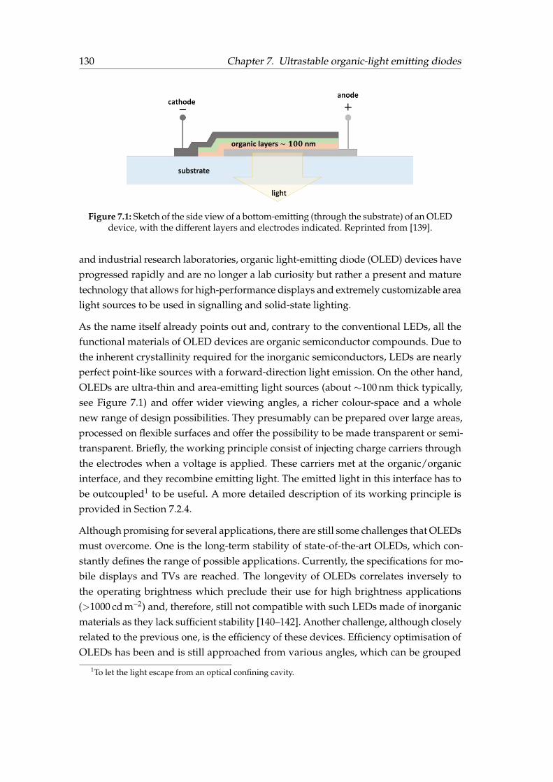
130 Chapter 7. Ultrastable organic-light emitting diodes
Figure 7.1: Sketch of the side view of a bottom-emitting (through the substrate) of an OLEDdevice, with the different layers and electrodes indicated. Reprinted from [139].
and industrial research laboratories, organic light-emitting diode (OLED) devices haveprogressed rapidly and are no longer a lab curiosity but rather a present and maturetechnology that allows for high-performance displays and extremely customizable arealight sources to be used in signalling and solid-state lighting.
As the name itself already points out and, contrary to the conventional LEDs, all thefunctional materials of OLED devices are organic semiconductor compounds. Due tothe inherent crystallinity required for the inorganic semiconductors, LEDs are nearlyperfect point-like sources with a forward-direction light emission. On the other hand,OLEDs are ultra-thin and area-emitting light sources (about ∼100 nm thick typically,see Figure 7.1) and offer wider viewing angles, a richer colour-space and a wholenew range of design possibilities. They presumably can be prepared over large areas,processed on flexible surfaces and offer the possibility to be made transparent or semi-transparent. Briefly, the working principle consist of injecting charge carriers throughthe electrodes when a voltage is applied. These carriers met at the organic/organicinterface, and they recombine emitting light. The emitted light in this interface has tobe outcoupled1 to be useful. A more detailed description of its working principle isprovided in Section 7.2.4.
Although promising for several applications, there are still some challenges that OLEDsmust overcome. One is the long-term stability of state-of-the-art OLEDs, which con-stantly defines the range of possible applications. Currently, the specifications for mo-bile displays and TVs are reached. The longevity of OLEDs correlates inversely tothe operating brightness which preclude their use for high brightness applications(>1000 cd m−2) and, therefore, still not compatible with such LEDs made of inorganicmaterials as they lack sufficient stability [140–142]. Another challenge, although closelyrelated to the previous one, is the efficiency of these devices. Efficiency optimisation ofOLEDs has been and is still approached from various angles, which can be grouped
1To let the light escape from an optical confining cavity.
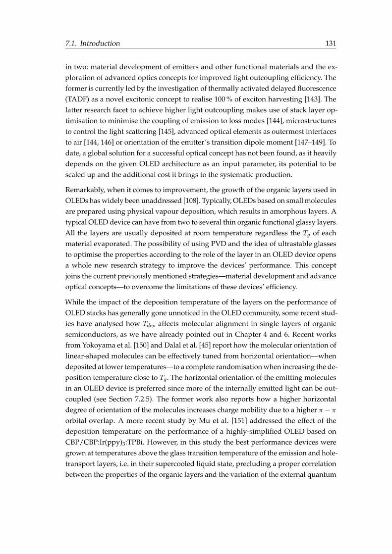
7.1. Introduction 131
in two: material development of emitters and other functional materials and the ex-ploration of advanced optics concepts for improved light outcoupling efficiency. Theformer is currently led by the investigation of thermally activated delayed fluorescence(TADF) as a novel excitonic concept to realise 100 % of exciton harvesting [143]. Thelatter research facet to achieve higher light outcoupling makes use of stack layer op-timisation to minimise the coupling of emission to loss modes [144], microstructuresto control the light scattering [145], advanced optical elements as outermost interfacesto air [144, 146] or orientation of the emitter’s transition dipole moment [147–149]. Todate, a global solution for a successful optical concept has not been found, as it heavilydepends on the given OLED architecture as an input parameter, its potential to bescaled up and the additional cost it brings to the systematic production.
Remarkably, when it comes to improvement, the growth of the organic layers used inOLEDs has widely been unaddressed [108]. Typically, OLEDs based on small moleculesare prepared using physical vapour deposition, which results in amorphous layers. Atypical OLED device can have from two to several thin organic functional glassy layers.All the layers are usually deposited at room temperature regardless the Tg of eachmaterial evaporated. The possibility of using PVD and the idea of ultrastable glassesto optimise the properties according to the role of the layer in an OLED device opensa whole new research strategy to improve the devices’ performance. This conceptjoins the current previously mentioned strategies—material development and advanceoptical concepts—to overcome the limitations of these devices’ efficiency.
While the impact of the deposition temperature of the layers on the performance ofOLED stacks has generally gone unnoticed in the OLED community, some recent stud-ies have analysed how Tdep affects molecular alignment in single layers of organicsemiconductors, as we have already pointed out in Chapter 4 and 6. Recent worksfrom Yokoyama et al. [150] and Dalal et al. [45] report how the molecular orientation oflinear-shaped molecules can be effectively tuned from horizontal orientation—whendeposited at lower temperatures—to a complete randomisation when increasing the de-position temperature close to Tg. The horizontal orientation of the emitting moleculesin an OLED device is preferred since more of the internally emitted light can be out-coupled (see Section 7.2.5). The former work also reports how a higher horizontaldegree of orientation of the molecules increases charge mobility due to a higher π − πorbital overlap. A more recent study by Mu et al. [151] addressed the effect of thedeposition temperature on the performance of a highly-simplified OLED based onCBP/CBP:Ir(ppy)3:TPBi. However, in this study the best performance devices weregrown at temperatures above the glass transition temperature of the emission and hole-transport layers, i.e. in their supercooled liquid state, precluding a proper correlationbetween the properties of the organic layers and the variation of the external quantum

132 Chapter 7. Ultrastable organic-light emitting diodes
efficiency. On the other hand, it should be pointed out that a frequent practice for solu-tion processed OLEDs is performing a thermal annealing after the preparation of theemissive layers, a procedure that has been previously shown to be effective in enhanc-ing the performance of polymer OLEDs [152]. However, vapour-deposition at temper-atures around 0.85Tg has demonstrated to be much more efficient than annealing inaccessing low energy positions in the potential energy landscape and consequently,achieveing glasses with enhanced stability and higher density [10].
In this work, we focus on the influence of ultrastable glass formation on two keyOLED performance indicators being the external quantum efficiency (EQE) and theoperational stability. First, and before presenting the OLED device and the results,we start by introducing some notions for organic semiconductors2 and organic light-emitting diodes. Here, we describe only the most basic and well-established conceptsof OLED science and technology that are necessary to build the framework in whichthe results are later discussed.
7.2 Organic semiconductors and OLEDs
The building blocks of organic semiconductors can be distinguished in two majorgroups: low-molecular weight materials and polymers. The most important and prac-tical difference between these two types of materials lies—for this work—in the wayin which they are processed as thin films. Whereas small molecules are prepared byPVD methods (generally vacuum evaporation), the conjugated polymers can only beprocessed from solution (e.g. spin coating or printing techniques). It is important tonote that when small molecules are vapour deposited, they yield amorphous layerswhich are—of course—the main reason for this study of OLEDs from the “glass physics”point of view. What all the organic semiconductors have in common is the origin oftheir “semiconductor” nature, which differs strongly from the inorganic’s.
7.2.1 Molecular orbitals
All the organic semiconductors have in common the conjugated π-electron systems,generally provided by the phenyl rings. A free carbon has an electronic structure of1s22s22p2. However, when this C atom is bound to other atoms, this configurationmight not be necessarily its optimal configuration. For instance, in benzene (Figure 7.2)the single carbon orbitals suffer the so-called hybridisation when the 2s and two of the2p orbitals mix forming the new sp2 orbitals, distributed in the xy plane with an angleof 120 between them. The remaining pz is orthogonal to that plane. The overlap of
2We will focus only on the most relevant features for organic light-emitting diodes, despite being afield that goes beyond this particular application (organic solar cells, organic transistors,. . . )
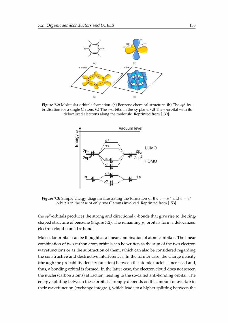
7.2. Organic semiconductors and OLEDs 133
Figure 7.2: Molecular orbitals formation. (a) Benzene chemical structure. (b) The sp2 hy-bridisation for a single C atom. (c) The σ-orbital in the xy plane. (d) The π-orbital with its
delocalized electrons along the molecule. Reprinted from [139].
Figure 7.3: Simple energy diagram illustrating the formation of the σ − σ∗ and π − π∗
orbitals in the case of only two C atoms involved. Reprinted from [153].
the sp2-orbitals produces the strong and directional σ-bonds that give rise to the ring-shaped structure of benzene (Figure 7.2). The remaining pz orbitals form a delocalizedelectron cloud named π-bonds.
Molecular orbitals can be thought as a linear combination of atomic orbitals. The linearcombination of two carbon atom orbitals can be written as the sum of the two electronwavefunctions or as the subtraction of them, which can also be considered regardingthe constructive and destructive interferences. In the former case, the charge density(through the probability density function) between the atomic nuclei is increased and,thus, a bonding orbital is formed. In the latter case, the electron cloud does not screenthe nuclei (carbon atoms) attraction, leading to the so-called anti-bonding orbital. Theenergy splitting between these orbitals strongly depends on the amount of overlap intheir wavefunction (exchange integral), which leads to a higher splitting between the

134 Chapter 7. Ultrastable organic-light emitting diodes
σ (bonding) and σ∗ (anti-bonding) states than between the π and π∗ states. This energysplitting is further illustrated in Figure 7.3 for the interaction of two carbon atoms. Inthis scenario, the highest occupied molecular orbital (HOMO) is a π-orbital. The followinghigher orbital is, therefore, the π∗ and is empty. This orbital is the so-called lowestunoccupied molecular orbital (LUMO). These delocalized π − π∗ orbitals are the mainlyresponsible ones for the electrical and optical properties of the organic semiconductormolecules. On the other hand, the stronger and directional covalent σ bonds are theones conferring most of the chemical properties to the molecule [153].
The energy gap between the HOMO and the LUMO is typically between 1.5 and 3.0eV, which leads to the absorption of light in the visible spectrum. This gap can becontrolled by the conjugation degree of the molecules. In that sense, chemistry offersa broad range of possibilities to synthesise different organic semiconductors with thedesired optoelectronic properties. These molecules are usually a group of phenyl rings,some 5 or 6-membered rings with some heteroatom—neither carbon nor hydrogen—such as nitrogen or sulphur together with alternated single and double bonds. Thefunction that a molecule will have on a device depends strongly on the HOMO/LUMOgap for the emission and absorption properties and the energy of these orbitals withrespect to the work function of the electrode material.
When using these organic semiconductors in OLEDs3, it is generally difficult to obtaina molecule that is efficient at the same time in emitting light, transporting electronsor transporting holes. In that sense, molecules are typically selected to accomplish itsbest convenient and specific function in an OLED device . For instance, molecules witha high quantum yield of luminescence are chosen as emitters, molecules that easilygive away electrons are used as hole transport layers (HTL) and molecules that easilyaccept electrons are used as electron transport layers (ETL).
7.2.2 Optical properties
Electrons and holes have a spin of s = 1/2. The total spin of an atomic/molecular stateis given basically for all the unpaired electrons in the orbitals since the filled orbitals donot contribute to the total spin. An excited state with one electron in the π∗-orbital andone electron in the π-orbital can have a S = 0 with anti-parallel electron spins (singlet)or S = 1 with both spins parallel (triplet). With the rules of quantum mechanics (alsoconsidering the z-component of the spin, Ms) we know that, in a two-particle system,there are four possible eigenstates; the singlet and the triplet, which can take threepossible values for the Ms component (1, 0 and -1).
3Other devices based on organic semiconductors can be fabricated, such as organic solar cells, organicfield-effect transistors or even organic lasers. Here we just focus on the specific application of thesematerials in organic light-emitting diodes.
7.2. Organic semiconductors and OLEDs 135
When an organic molecule is excited, either optically or electrically, an exciton—a pairof electron-hole bounded by Coulomb interaction—is formed. These excitons can endup either in a singlet or triplet state. Statistically, a ratio of 3:1 of triplets to singlets statesare formed during an electric excitation. On the other hand, since the ground state isa singlet and due to the spin conservation rules, only transitions from singlet statesto the ground state are allowed. That means that transitions from the triplet statesto the ground are forbidden. However, these kind of transitions are experimentallyobserved, a process referred as phosphorescence in distinction to the singlet to singlettransition known as fluorescence. This is because “forbidden” is used in the quantum-mechanical sense, i.e. the probability of phosphorescence to happen is, generally, ordersof magnitude lower than fluorescence which, in practice, means that the lifetime ofphosphorescence is much longer. The ratio of optically excited singlet/triplet states inorganic materials can be as high as 109-1010 to 1 [154].
A mechanism that weakens the spin selection rules and, therefore, allows an efficientphosphorescence is the spin-orbit coupling, which induces a mixing of the singlet andtriplet states. Since it is the total angular momentum (orbital plus spin) what must beconserved, this mechanism can flip the spin of the electron at expenses of also chang-ing the orbital momentum. However, the spin-orbit coupling is minimal in low atomicmass elements and cannot provide an efficient radiative relaxation from the triplet tothe singlet state that must, instead, relax to nonradiative processes (vibrational mainly)[153]. An OLED device based only on fluorescence would be rather inefficient sinceonly 25 % of the excitons would be allowed to decay radiatively because the emissionwould only take place from the singlet state, as sketched in Figure 7.4. For few yearsalready, this limitation has been overcome by the incorporation of phosphorescentemitters to the organic matrix at low-concentrations [155] to avoid the so-called triplet-triplet annihilation4. These materials consist of organometallic complexes with a heavymetal atom in their core (e.g. platinum or iridium) enhancing the spin-orbit coupling,which implies that these molecules can effectively emit from the triplet state (phospho-rescence). Moreover, the intersystem crossing (ISC) rate—transitions with a change ofspin involved—between the singlet and the triplet is also increased. That means thatthe fraction of the singlets created by electrical excitation is converted to triplets beforethey radiatively decay. In such a way, the phosphorescent OLEDs have a total inter-nal electroluminescent efficiency of 100 %, instead of the 25 % of fluorescence-basedOLEDs. Figure 7.4 sums up the different and most important radiative and nonra-diative transitions within an excited molecule. Notice that an additional splitting ofthe main levels is also drawn, which corresponds to the vibrational states, typicallyexhibiting a factor of 10 lower energy differences.
4The interaction of two triplet excitons that can lead to the annihilation of the these and that must beavoided.
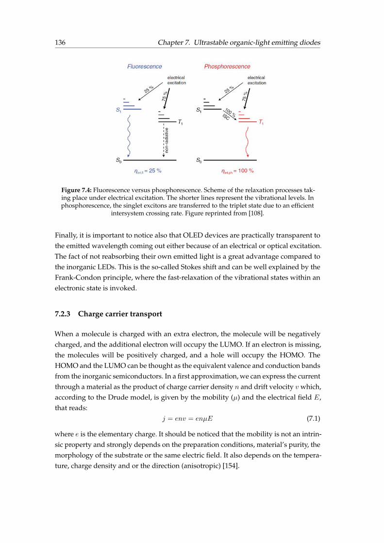
136 Chapter 7. Ultrastable organic-light emitting diodes
Figure 7.4: Fluorescence versus phosphorescence. Scheme of the relaxation processes tak-ing place under electrical excitation. The shorter lines represent the vibrational levels. Inphosphorescence, the singlet excitons are transferred to the triplet state due to an efficient
intersystem crossing rate. Figure reprinted from [108].
Finally, it is important to notice also that OLED devices are practically transparent tothe emitted wavelength coming out either because of an electrical or optical excitation.The fact of not reabsorbing their own emitted light is a great advantage compared tothe inorganic LEDs. This is the so-called Stokes shift and can be well explained by theFrank-Condon principle, where the fast-relaxation of the vibrational states within anelectronic state is invoked.
7.2.3 Charge carrier transport
When a molecule is charged with an extra electron, the molecule will be negativelycharged, and the additional electron will occupy the LUMO. If an electron is missing,the molecules will be positively charged, and a hole will occupy the HOMO. TheHOMO and the LUMO can be thought as the equivalent valence and conduction bandsfrom the inorganic semiconductors. In a first approximation, we can express the currentthrough a material as the product of charge carrier density n and drift velocity v which,according to the Drude model, is given by the mobility (µ) and the electrical field E,that reads:
j = env = enµE (7.1)
where e is the elementary charge. It should be noticed that the mobility is not an intrin-sic property and strongly depends on the preparation conditions, material’s purity, themorphology of the substrate or the same electric field. It also depends on the tempera-ture, charge density and or the direction (anisotropic) [154].
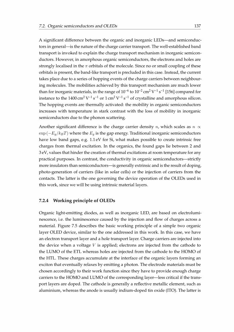
7.2. Organic semiconductors and OLEDs 137
A significant difference between the organic and inorganic LEDs—and semiconduc-tors in general—is the nature of the charge carrier transport. The well-established bandtransport is invoked to explain the charge transport mechanism in inorganic semicon-ductors. However, in amorphous organic semiconductors, the electrons and holes arestrongly localised in the π orbitals of the molecule. Since no or small coupling of theseorbitals is present, the band-like transport is precluded in this case. Instead, the currenttakes place due to a series of hopping events of the charge carriers between neighbour-ing molecules. The mobilities achieved by this transport mechanism are much lowerthan for inorganic materials, in the range of 10−6 to 10−2 cm2 V−1 s−1 [156] compared forinstance to the 1400 cm2 V−1 s−1 or 1 cm2 V−1 s−1 of crystalline and amorphous silicon.The hopping events are thermally activated: the mobility in organic semiconductorsincreases with temperature in stark contrast with the loss of mobility in inorganicsemiconductors due to the phonon scattering.
Another significant difference is the charge carrier density n, which scales as n ∝exp (−Eg/kBT ) where the Eg is the gap energy. Traditional inorganic semiconductorshave low band gaps, e.g. 1.1 eV for Si, what makes possible to create intrinsic freecharges from thermal excitation. In the organics, the found gaps lie between 2 and3 eV, values that hinder the creation of thermal excitations at room temperature for anypractical purposes. In contrast, the conductivity in organic semiconductors—strictlymore insulators than semiconductors—is generally extrinsic and is the result of doping,photo-generation of carriers (like in solar cells) or the injection of carriers from thecontacts. The latter is the one governing the device operation of the OLEDs used inthis work, since we will be using intrinsic material layers.
7.2.4 Working principle of OLEDs
Organic light-emitting diodes, as well as inorganic LED, are based on electrolumi-nescence, i.e. the luminescence caused by the injection and flow of charges across amaterial. Figure 7.5 describes the basic working principle of a simple two organiclayer OLED device, similar to the one addressed in this work. In this case, we havean electron transport layer and a hole transport layer. Charge carriers are injected intothe device when a voltage V is applied; electrons are injected from the cathode tothe LUMO of the ETL whereas holes are injected from the cathode to the HOMO ofthe HTL. These charges accumulate at the interface of the organic layers forming anexciton that eventually relaxes by emitting a photon. The electrode materials must bechosen accordingly to their work function since they have to provide enough chargecarriers to the HOMO and LUMO of the corresponding layer—less critical if the trans-port layers are doped. The cathode is generally a reflective metallic element, such asaluminium, whereas the anode is usually indium-doped tin oxide (ITO). The latter is

138 Chapter 7. Ultrastable organic-light emitting diodes
Figure 7.5: OLED device working principle. The electroluminescence is achieved whena voltage is applied across the electrodes allowing the injection of holes and electrons tothe HOMO and LUMO levels of the respective organic layers. Those form an exciton that
recombines radiatively.
the most commonly used anode material for OLEDs since it is conductive and transpar-ent at the same time. Therefore, the produced light of the OLED is outcoupled throughthe transparent ITO anode. Due to its semiconductor nature, OLED devices exhibitcurrent-voltage curves with diode-like characteristics.
As mentioned before, current OLEDs have normally incorporated phosphorescent emit-ters so they can emit efficiently from the triplet state. In practice and in short, this isachieved by introducing an emission layer (EML) between the ETL and HTL. Thislayer consists of a matrix material (can be the same material as the electron or holetransport layers) doped with a small concentration (generally less than 10 wt%) of anorganometallic complex and is usually about few nanometres thick. Current OLEDdevices can be far more complex than the one depicted in Figure 7.5. They can havedoped HTL/ETL layers, additional functional layers such as hole and electron blockinglayers, multiple emission layers for white OLEDs, among other functional layers [7].
7.2.5 Light outcoupling
It is of fundamental importance to assess which fraction of all the photons producedinside an OLED (generated in the emission layer) can escape to the air. Figure 7.6shows a scheme of the side view of an OLED including the glass substrate. In this case,the emission takes place through the substrate—meaning that the transparent anodeis the first deposited layer. This device geometry is called bottom-emitting (like theones prepared in this work). The different refractive indices of the layers are indicatedin Figure 7.6. The organic functional layers are not distinguished since they exhibitvery similar refractive indices, which can change from 1.7 to 2.1 depending on thewavelength.
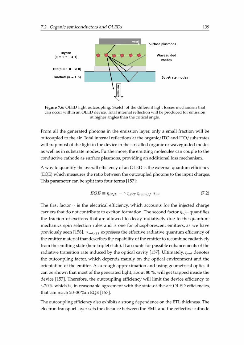
7.2. Organic semiconductors and OLEDs 139
Figure 7.6: OLED light outcoupling. Sketch of the different light losses mechanism thatcan occur within an OLED device. Total internal reflection will be produced for emission
at higher angles than the critical angle.
From all the generated photons in the emission layer, only a small fraction will beoutcoupled to the air. Total internal reflections at the organic/ITO and ITO/substrateswill trap most of the light in the device in the so-called organic or waveguided modesas well as in substrate modes. Furthermore, the emitting molecules can couple to theconductive cathode as surface plasmons, providing an additional loss mechanism.
A way to quantify the overall efficiency of an OLED is the external quantum efficiency(EQE) which measures the ratio between the outcoupled photons to the input charges.This parameter can be split into four terms [157]:
EQE ≡ ηEQE = γ ηS/T ηrad,eff ηout (7.2)
The first factor γ is the electrical efficiency, which accounts for the injected chargecarriers that do not contribute to exciton formation. The second factor ηS/T quantifiesthe fraction of excitons that are allowed to decay radiatively due to the quantum-mechanics spin selection rules and is one for phosphorescent emitters, as we havepreviously seen [158]. ηrad,eff expresses the effective radiative quantum efficiency ofthe emitter material that describes the capability of the emitter to recombine radiativelyfrom the emitting state (here triplet state). It accounts for possible enhancements of theradiative transition rate induced by the optical cavity [157]. Ultimately, ηout denotesthe outcoupling factor, which depends mainly on the optical environment and theorientation of the emitter. As a rough approximation and using geometrical optics itcan be shown that most of the generated light, about 80 %, will get trapped inside thedevice [157]. Therefore, the outcoupling efficiency will limit the device efficiency to∼20 % which is, in reasonable agreement with the state-of-the-art OLED efficiencies,that can reach 20–30 %in EQE [157].
The outcoupling efficiency also exhibits a strong dependence on the ETL thickness. Theelectron transport layer sets the distance between the EML and the reflective cathode

140 Chapter 7. Ultrastable organic-light emitting diodes
Figure 7.7: Effect of the orientation of transition dipoles. Sketch of the effect of the orienta-tion of the dipoles as a function of its orientation. The direction of the transition dipole ismarked by the dark-red thicker arrow, whereas the length of light-red arrow indicates the
direction and strength of the emitted radiation.
which, in the end, determines the resonant conditions inside the OLED cavity becauseof the interferences—constructive and destructive—of the light waves. For that rea-son, optical simulations are performed to determine the optimal thicknesses of thefunctional layers. The OLEDs are built in their first (as in this work) or second opticalmaximum.
7.2.6 Orientation of the emitting dipoles
The orientation of the transition dipoles (where the emission takes place) strongly influ-ences the outcoupling efficiency. In an OLED device, a horizontal dipole orientation ofthe emitting molecules is preferred. There are two main reasons for that. In Figure 7.7we can see how vertical dipoles emit light preferentially at higher angles with respectto the substrate normal, which will suffer total internal reflections and will be coupledto waveguide modes. On the other hand, horizontal dipoles emit light preferentiallyat lower angles with respect to the substrate normal allowing, therefore, more lightcan be directly outcoupled. Additionally, vertical dipoles only emit p-polarized lightwhereas horizontal dipoles have the contribution of both p-polarized and s-polarizedlight. Only the p-polarized modes can couple to surface plasmons modes; therefore,horizontal orientation is preferred, so more s-polarized modes contribute to the lightoutcoupling [157].
As we have seen in the previous chapter, physical vapour deposition can be used totune the orientation of the molecules by changing the deposition temperature. Thisstrategy could offer new possibilities to enhance the outcoupling efficiency of OLEDdevices.

7.3. Experimental 141
7.3 Experimental
In this section, both the preparation and characterisation of the OLED devices studiedin this work is explained. It is important to note that the devices were prepared andcharacterized at the IAPP in Dresden. We provide here a description of the fabricationprocess and of the specific techniques used to characterize the device. The sampleswere prepared in a highly-standardised evaporation tool at the IAPP which ensuresthe proper reproducibility of the devices.
7.3.1 Sample preparation
Glass substrates (Corning Eagle XG, Thin Films devices, Inc.) with a thickness of1.1 mm and with 90 nm of pre-deposited ITO as a transparent bottom electrode fol-lowed a standard cleaning procedure (including rinsing with NMP, ethanol and de-ionised water as well as treatment with UV ozone). The ITO is patterned in a sucha structure that will allow the creation of four independent pixels in each one of the25× 25 mm2 substrates. Figure 7.8 shows an image of a final OLED were the fourpixels can be seen.
All the subsequent layers were deposited in a single vacuum chamber evaporation tool(Kurt J. LESKER & Co.) at a base pressure of 10−7 mbar. In a single evaporation run, a150× 150 mm2 wafer, patterned with the 25× 25 mm2 ITO-contacts, is used, allowingto obtain up to 36 OLED devices with four (identical) pixels each one. The use of differ-ent wedge tools makes possible to individually address each column/row, obtainingdifferent samples in a single run. The substrate rotates during the evaporation to en-sure a homogeneous layer thickness. The structuring of the different evaporated layersis achieved using shadow masks.
The thickness and deposition rates were monitored using a quartz crystal microbal-ance. The evaporation tool has up to 12 organic sources plus three other metal sources.This tool allows to evaporate the whole device structure in a single run and performco-evaporation for the mixed layers. First, a 0.5 nm thin layer of MoO3 was evapo-rated on top of the ITO to facilitate the injection of the holes into the cathode. Theelectrode is followed by the two organic layers TCTA and TPBi, as hole transport andelectron transport layers, respectively (see Section 2.1.6 for full names). The emissionlayer (EML) was formed by doping the first part of the ETL layer with the respectivephosphorescent dopant (later described). Additionally, four different phosphorescentemitters were tested, with the remaining stack architecture kept identical. For all emit-ters, the layer thicknesses of HTL and ETL were optimised using a thin film opticssimulation tool [159], which also considered the transition dipole moment orientation.Different samples were prepared by changing only the substrate temperature during
142 Chapter 7. Ultrastable organic-light emitting diodes
Figure 7.8: Photographs of the prepared OLED devices. In the left picture (device off), thefour pixels can be seen. In the right, the central to pixels have been turned on.
the evaporation of the EML and ETL layers for each of the mentioned devices to studythe effect of the TPBi layer’s properties on the device performance. Finally, a bilayercathode consisting of 0.5 nm of LiF/ aluminium was deposited on top of the organiclayers. The overlap between the ITO contact and the aluminium cathode defines theactive area of each pixel which is, in our case, of 6.49 mm2.
The OLEDs are highly sensitive to air and moisture. For that reason, a glove box undera nitrogen atmosphere is directly coupled to the evaporation chamber where, immedi-ately after fabrication, all OLEDs are encapsulated with glass lids with a small cavityto prevent the direct contact. Once finished, the glass wafer is cut to obtain the 36individual samples.
In the first studied device, referred from now on as G0, the precise structure was asfollows: ITO (90 nm) / MoO3 (0.5 nm) / TCTA (64 nm) / TPBi:Ir(ppy)2(acac) 8 wt%(10 nm) / TPBi (60 nm) / LiF (0.5 nm) / Al (100 nm), where Ir(ppy)2(acac) 5 is a greenphosphorescent emitter dopant. After depositing the HTL layer, the temperature ofthe whole substrate was radiatively heated and set to the highest temperature studied,90 C, where the EML and ETL were evaporated to a limited area (a column of sixsamples) using the wedge tool. After reaching the next temperature (another column)by passively cooling the whole substrate, the EML and ETL were evaporated againinto another predefined region. This procedure was repeated six times (one for eachcolumn) at the nominal temperatures of 90 C, 80 C, 70 C, 60 C, 50 C and room tem-perature (ca. 30 C). A previously performed calibration determined the real substratetemperature. Once room temperature is reached, the cathode layers were evaporatedat once for all the samples.
The other set of three different devices was prepared using the same structure andchanging only the emitter—i.e. using same electrode scheme and with the HTL andETL thicknesses optimised for each emitter spectra. All three devices were prepared in
5Full name: bis(2-phenylpyridine) (acetylacetonate)iridium(III)

7.3. Experimental 143
a single run by using shadow masks. The structure of these three devices summarisedby Table 7.1 and will be referred as device R1 for the red emitter Ir(MDQ)2(acac)6,device G1 for the new green emitter Ir(ppy)3
7 and device B1 for the blue emitter FIrpic8.
device Hole transport layer Emission layer Electron transport layerTCTA TPBi:emitter TPBi
G0 64 nm 10 nm 60 nmIr(ppy)2(acac) 8 wt%
R1 90 nm 10 nm 70 nmIr(MDQ)2(acac) 10 wt%
G1 64 nm 10 nm 60 nmIr(ppy)3 10 wt%
B1 40 nm 10 nm 35 nmFIrpic 10 wt%
Table 7.1: Device architecture of all the devices studied in this chapter. The thickness ofthe electrode and injection layers are the same in all cases and reported in the text.
Based on the results obtained from the G0 device, for each one of the three devices, R1,G1 and B1, two deposition temperatures for the EML and ETL layers were explored:room temperature and 66 C using the aforementioned procedure.
7.3.2 OLED characterization
The basic OLED characterisation is based mainly on three quantities: current density,voltage and luminance—or, equivalently, brightness. While the former two do notneed any clarification, the luminance requires a brief introduction. The radiance of alight source is a measure of the radiant power (Φr), per unit of solid angle and unit ofprojected area:
Lr =d2Φr
dΩdAsource cosϑ
[W sr−1 m−2
](7.3)
which is a so-called radiometric quantity. However, organic LED, as well as other light-emitting sources, are generally characterised by photometric quantities. Contrary toradiometry, photometry considers the human eye sensitivity to the light and weightsthe different wavelengths according to it. In analogy to the radiometric radiant power(units Watts), the equivalent photometric quantity is defined as luminous flux Φph
(units Lumen or lm). Both quantities are related by
dΦr
dλ= KmV (λ)
dΦph
dλ(7.4)
6Full name: Bis(2-methyldibenzo[f,h]quinoxaline)(acetylacetonate)iridium(III)7Full name: Tris[2-phenylpyridine]iridium(III)8Full name: Bis[2-(4,6-difluorophenyl)pyridinato-C2,N](picolinato)iridium(III)
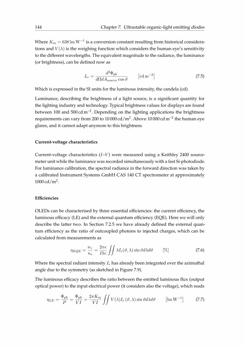
144 Chapter 7. Ultrastable organic-light emitting diodes
Where Km = 638 lm W−1 is a conversion constant resulting from historical considera-tions and V (λ) is the weighing function which considers the human eye’s sensitivityto the different wavelengths. The equivalent magnitude to the radiance, the luminance(or brightness), can be defined now as
Lr =d2Φph
dΩdAsource cosϑ
[cd m−2
](7.5)
Which is expressed in the SI units for the luminous intensity, the candela (cd).
Luminance, describing the brightness of a light source, is a significant quantity forthe lighting industry and technology. Typical brightness values for displays are foundbetween 100 and 500 cd m−2. Depending on the lighting applications the brightnessrequirements can vary from 200 to 10 000 cd/m2. Above 10 000 cd m−2 the human eyeglares, and it cannot adapt anymore to this brightness.
Current-voltage characteristics
Current-voltage characteristics (I–V ) were measured using a Keithley 2400 source-meter unit while the luminance was recorded simultaneously with a fast Si-photodiode.For luminance calibration, the spectral radiance in the forward direction was taken bya calibrated Instrument Systems GmbH CAS 140 CT spectrometer at approximately1000 cd/m2.
Efficiencies
OLEDs can be characterised by three essential efficiencies: the current efficiency, theluminous efficacy (LE) and the external quantum efficiency (EQE). Here we will onlydescribe the latter two. In Section 7.2.5 we have already defined the external quan-tum efficiency as the ratio of outcoupled photons to injected charges, which can becalculated from measurements as
ηEQE =nγne
=2πe
Ihc
∫∫λIe(ϑ, λ) sinϑdλdϑ [%] (7.6)
Where the spectral radiant intensity Ie has already been integrated over the azimuthalangle due to the symmetry (as sketched in Figure 7.9).
The luminous efficacy describes the ratio between the emitted luminous flux (outputoptical power) to the input electrical power (it considers also the voltage), which reads
ηLE =Φph
P=
Φph
V I=
2πKm
V I
∫∫V (λ)Ie (ϑ, λ) sinϑdλdϑ
[lm W−1] (7.7)

7.3. Experimental 145
Figure 7.9: The geometry of the OLED allows only the emission through the forwardhemisphere since the backwards emission is blocked by the metallic electrode. The polarcoordinates are used to calculate the total EQE and LE using the integrating sphere setup.
The azimuthal angle is given already integrated in equations 7.6 and 7.7.
Since it is a photometric quantity, it includes the aforementioned weighting functionfor the human eye.
Both integral terms in equation 7.6 and 7.7 can be obtained at a constant current usingan integrating sphere. In such system, the spectral emission in all directions (into theforward half space due to the OLED geometry, see Figure 7.9) of an OLED is captured,which allows obtaining the integral term experimentally. Therefore, the EQE and LEare measured at only one current value, corresponding approximately to 1000 cd m−2.To these values for the whole j range we proceed as follows:
(i) Our OLED does not exhibit any colour shift at different currents (same spectra)and is planar. Therefore, we assume that the spectral radiant intensity (over allangles) is constant for all currents.
(ii) The EQE and LE curves as a function of the current are obtained from the lumi-nance (defined for forward direction) of the previous j–V –L characterisation andassuming a lambertian emitter 9, i.e. (Ie = I0e cosϑ).
(iii) The measurement at the integrating sphere allows correcting the EQE for the non-lambertian characteristics of the OLED. The scale factor obtained from the twoEQE values (from the lambertian assumption and integrating-sphere measure-ment) at 1000 cd m−2 is applied to the whole current range.
In this work, an integrating sphere (LMS-100 Labsphere Inc.) with a calibrated spec-trometer (CDS-600, Labsphere Inc) was used. For each deposition temperature, the datafrom two to four identically prepared devices, having four distinct pixels each, wereaveraged. The error bars correspond to the standard deviation with 95 % confidenceinterval corrected by the t-student factor for a small number of samples.
9Which states that the radiant intensity directly observed from the emission area is proportional tocosϑ, where ϑ is the angle between the surface normal and the direction of the incident light.
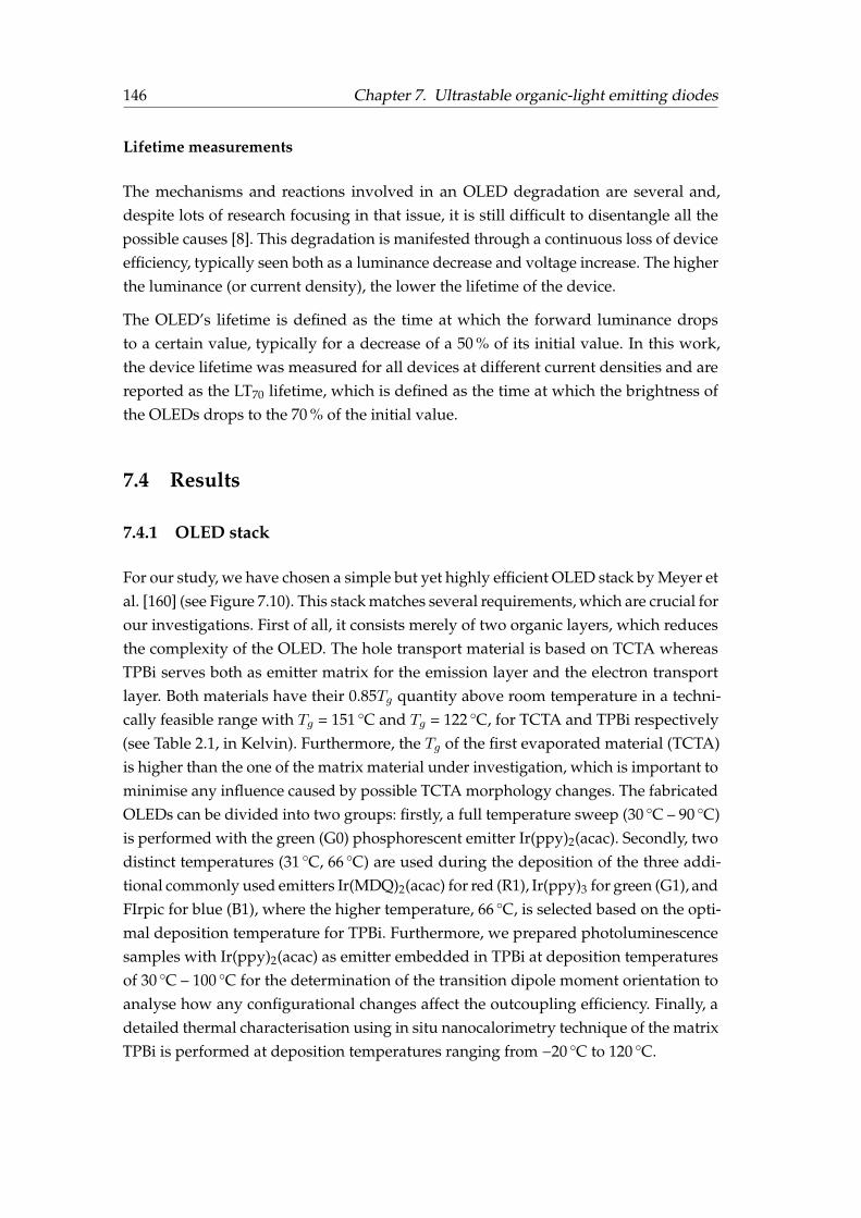
146 Chapter 7. Ultrastable organic-light emitting diodes
Lifetime measurements
The mechanisms and reactions involved in an OLED degradation are several and,despite lots of research focusing in that issue, it is still difficult to disentangle all thepossible causes [8]. This degradation is manifested through a continuous loss of deviceefficiency, typically seen both as a luminance decrease and voltage increase. The higherthe luminance (or current density), the lower the lifetime of the device.
The OLED’s lifetime is defined as the time at which the forward luminance dropsto a certain value, typically for a decrease of a 50 % of its initial value. In this work,the device lifetime was measured for all devices at different current densities and arereported as the LT70 lifetime, which is defined as the time at which the brightness ofthe OLEDs drops to the 70 % of the initial value.
7.4 Results
7.4.1 OLED stack
For our study, we have chosen a simple but yet highly efficient OLED stack by Meyer etal. [160] (see Figure 7.10). This stack matches several requirements, which are crucial forour investigations. First of all, it consists merely of two organic layers, which reducesthe complexity of the OLED. The hole transport material is based on TCTA whereasTPBi serves both as emitter matrix for the emission layer and the electron transportlayer. Both materials have their 0.85Tg quantity above room temperature in a techni-cally feasible range with Tg = 151 C and Tg = 122 C, for TCTA and TPBi respectively(see Table 2.1, in Kelvin). Furthermore, the Tg of the first evaporated material (TCTA)is higher than the one of the matrix material under investigation, which is important tominimise any influence caused by possible TCTA morphology changes. The fabricatedOLEDs can be divided into two groups: firstly, a full temperature sweep (30 C – 90 C)is performed with the green (G0) phosphorescent emitter Ir(ppy)2(acac). Secondly, twodistinct temperatures (31 C, 66 C) are used during the deposition of the three addi-tional commonly used emitters Ir(MDQ)2(acac) for red (R1), Ir(ppy)3 for green (G1), andFIrpic for blue (B1), where the higher temperature, 66 C, is selected based on the opti-mal deposition temperature for TPBi. Furthermore, we prepared photoluminescencesamples with Ir(ppy)2(acac) as emitter embedded in TPBi at deposition temperaturesof 30 C – 100 C for the determination of the transition dipole moment orientation toanalyse how any configurational changes affect the outcoupling efficiency. Finally, adetailed thermal characterisation using in situ nanocalorimetry technique of the matrixTPBi is performed at deposition temperatures ranging from −20 C to 120 C.
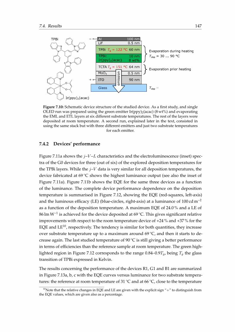
7.4. Results 147
Figure 7.10: Schematic device structure of the studied device. As a first study, and singleOLED run was prepared using the green emitter Ir(ppy)2(acac) (8 wt%) and evaporatingthe EML and ETL layers at six different substrate temperatures. The rest of the layers weredeposited at room temperature. A second run, explained later in the text, consisted inusing the same stack but with three different emitters and just two substrate temperatures
for each emitter.
7.4.2 Devices’ performance
Figure 7.11a shows the j–V –L characteristics and the electroluminescence (inset) spec-tra of the G0 devices for three (out of six) of the explored deposition temperatures forthe TPBi layers. While the j–V data is very similar for all deposition temperatures, thedevice fabricated at 69 C shows the highest luminance output (see also the inset ofFigure 7.11a). Figure 7.11b shows the EQE for the same three devices as a functionof the luminance. The complete device performance dependence on the depositiontemperature is summarised in Figure 7.12, showing the EQE (red-squares, left-axis)and the luminous efficacy (LE) (blue-circles, right-axis) at a luminance of 100 cd m−2
as a function of the deposition temperature. A maximum EQE of 24.0 % and a LE of86 lm W−1 is achieved for the device deposited at 69 C. This gives significant relativeimprovements with respect to the room temperature device of +24 % and +37 % for theEQE and LE10, respectively. The tendency is similar for both quantities, they increaseover substrate temperature up to a maximum around 69 C, and then it starts to de-crease again. The last studied temperature of 90 C is still giving a better performancein terms of efficiencies than the reference sample at room temperature. The green high-lighted region in Figure 7.12 corresponds to the range 0.84–0.9Tg, being Tg the glasstransition of TPBi expressed in Kelvin.
The results concerning the performance of the devices R1, G1 and B1 are summarizedin Figure 7.13a, b, c with the EQE curves versus luminance for two substrate tempera-tures: the reference at room temperature of 31 C and at 66 C, close to the temperature
10Note that the relative changes in EQE and LE are given with the explicit sign “+” to distinguish fromthe EQE values, which are given also as a percentage.
148 Chapter 7. Ultrastable organic-light emitting diodes
Figure 7.11: Optoelectronic characterisation of device G0. (a) j–V and L–V characteristicsof the G0 devices prepared at three different substrate temperatures: 32 C (room tem-perature), 69 C and 90 C, the other three temperatures are not shown for clarity. Eachcurve is the mean of 2-6 pixels. (b) External quantum efficiency characteristics for thesame three different temperatures over luminance for the G0 devices. The shadowed arearepresents the errobars, which are the standard deviation at the 95 % confidence intervaland weighted with the t-student factor for small samples sizes (between two to six pixel
for each temperature).
with the best performance for the G0 device. The electroluminescence spectra obtainedin an integrating sphere are shown for a current density of 15.4 mA cm−2 and sameintegration time in Figure 7.13d, e, f. In all three devices, there is a significant enhance-ment between the reference device prepared at room temperature and the device with

7.4. Results 149
Figure 7.12: Devices performance versus deposition temperature. External quantum effi-ciency (EQE) (red, left-axis) and luminous efficacy (LE) (blue, right-axis) at 100 cd m−2 asa function of the deposition temperature. The errorbars are the standard deviation at the95 % confidence interval and weighted with the t-student factor for small samples sizes
(between 2 and 6 samples for each temperature). Lines are a guide-to-the-eyes.
the ETL and EML deposited at 66 C. The EQE enhancements over the respective ref-erence OLEDs at 100 cd m−2 are +14.5 % for the red R1 devices, +21.7 % for the greenG1 devices, and +165 % for the blue B1 devices. All devices fabricated at 66 C showan increased phosphorescence lifetime of 1.16 to 1.36 µs (+17 % increase) for R1, 0.87to 1.00 µs (+15 %) for G1, and 1.07 to 1.38 µs (+29 %) for B1, as obtained from photolu-minescence spectroscopy of the complete OLEDs (see Figure 7.13g, h, i). The j–V –Lcurves of all devices R1, G1, and B1 can be found in the Appendix A.
7.4.3 Lifetime
Figure 7.14 shows an example of lifetime curves for luminance (left-axis) and voltage(right-axis). Figure 7.15 summarises the device lifetimes LT70 (i.e. time to reach 70 % ofinitial luminance) for the green devices G0, G1 and the red device R1 at various currentdensities. For G0 at 5 and 10 mA cm−2, we find in average the highest LT70 at a substratetemperature of 59 C (0.84Tg). This is an enhancement compared to room temperatureof +41 % (7.98 h versus 5.65 h) and +11 % (2.63 h versus 2.36 h), respectively. Similarly,for G1 and R1, the LT70 peaks for all investigated current densities at 66 C. Even at30 mA cm−2 an enhancement of +14 % is found for G1 (0.49 h versus 0.43 h) and +58 %for R1 (2.72 h versus 1.72 h). Similar to the correlation of the device efficiency values,the different maxima in device lifetimes are coinciding with the substrate temperature

150 Chapter 7. Ultrastable organic-light emitting diodes
Figure 7.13: Performance characteristics for different phosphorescent emitters and differ-ent deposition temperatures. External quantum efficiency (a-c), electroluminescence (d-f)and photoluminescence lifetime (g-i) for the devices R1, G1 and B1, which only differ in theemitter respect to the G0 stack. (a), (d) and (c) OLED with the red emitter (Ir(MDQ)2(acac)).(b), (e) and (h) OLED with a second green emitter Ir(ppy)3 and (c), (f) and (i) OLED withthe blue emitter (FIrpic). For each different emitter two deposition temperatures werestudied; room temperature (31 C) and 66 C. The arrow with the label indicates the EQE
improvement respect the RT devices at a luminance of 100 cd m−2 in all three cases.
range for the formation of ultrastable glasses. The lifetime of the blue device series B1was not evaluated because the emitter FIrpic has only a very short intrinsic stabilitynot allowing for a sound analysis [142]. A summary of the devices’ performance (EQEand LT70) is given in Table 7.2.
7.5 Discussion
As seen in Figure 7.12 and Figure 7.14, the deposition temperature at which the ETLand EML layers are evaporated has a clear impact on the device’s performance (forboth efficiency and lifetime). For instance, looking at the EQE as a benchmark effi-ciency, it can be enhanced from 19.4 % to 24.0 % between the room temperature andthe 69 C G0 devices. When trying to understand the origin of this improvement, we

7.5. Discussion 151
Figure 7.14: Example of OLED R1 lifetime and voltage over ageing time. Decreased lumi-nance and increase voltage for a constant current density of 10 mA cm−2 for the R1 devices
evaporated at 30 C (a) and 65 C (b), respectively. The LT70 is enhanced by 54 %.
Figure 7.15: Device lifetimes at different current densities as a function of the depositiontemperature. The lifetime LT70 is defined as the time it takes for the initial luminance todrop to 70 %. Lower current densities j lead to higher lifetimes, e.g. the bars with lower jare mostly hidden by bars with higher j. For G0, G1 and R1 we find enhanced LT70 for allcurrent densities at the temperature close to 0.85Tg (solid bars), except for 30 mA cm−2 forG0. Device B1 could not be measured because of the very unstable blue emitter FIrpic. Theerrorbars account for identical measurements setup (e.g. j, Tdep) of devices. If no errorbar
is given, the measurement is unique.
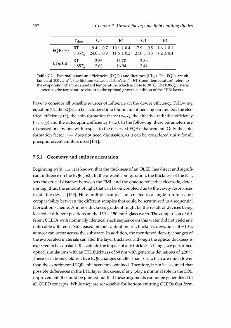
152 Chapter 7. Ultrastable organic-light emitting diodes
Tdep G0 R1 G1 B1
EQE (%)RT 19.4± 0.7 10.1± 0.4 17.9± 0.5 1.6± 0.10.85Tg 24.0± 0.9 11.6± 0.2 21.8± 0.5 4.2± 0.4
LT70 (h)RT 2.36 11.70 2.89 –0.85Tg 2.63 16.94 3.48 –
Table 7.2: . External quantum efficiencies (EQEs) and lifetimes (LT70). The EQEs are ob-tained at 100 cd m−2, the lifetime values at 10 mA cm−2. RT (room temperature) refers tothe evaporation chamber standard temperature, which is close to 30 C. The 0.85Tg criteria
refers to the temperature closest to the optimal growth condition of the TPBi layers.
have to consider all possible sources of influence on the device efficiency. Followingequation 7.2, the EQE can be factorized into four main influencing parameters: the elec-trical efficiency (γ), the spin formation factor (ηS/T ), the effective radiative efficiency(ηrad,eff ) and the outcoupling efficiency (ηout). In the following, these parameters arediscussed one by one with respect to the observed EQE enhancement. Only the spinformation factor ηS/T does not need discussion, as it can be considered unity for allphosphorescent emitters used [161].
7.5.1 Geometry and emitter orientation
Beginning with ηout, it is known that the thickness of an OLED has direct and signifi-cant influence on the EQE [162]. In the present configuration, the thickness of the ETLsets the crucial distance between the EML and the opaque reflective electrode, deter-mining, thus, the amount of light that can be outcoupled due to the cavity resonancesinside the device [159]. Here multiple samples are created in a single run to assurecomparability between the different samples that could be scrutinized in a sequentialfabrication scheme. A minor thickness gradient might be the result of devices beinglocated at different positions on the 150× 150 mm2 glass wafer. The comparison of dif-ferent OLEDs with nominally identical stack sequence on this wafer did not yield anynoticeable difference. Still, based on tool calibration test, thickness deviations of ±10 %at most can occur across the substrate. In addition, the mentioned density changes ofthe evaporated materials can alter the layer thickness, although the optical thickness isexpected to be constant. To evaluate the impact of any thickness change, we performedoptical simulations with an ETL thickness of 60 nm with generous deviations of±20 %.These variations yield relative EQE changes smaller than 5 %, which are much lowerthan the experimental EQE enhancements obtained. Therefore, it can be assumed thatpossible differences in the ETL layer thickness, if any, play a minimal role in the EQEimprovement. It should be pointed out that these arguments cannot be generalized toall OLED concepts. While they are reasonable for bottom-emitting OLEDs that form

7.5. Discussion 153
a weak optical cavity 11, top-emitting or cavity enhanced designs will be much moresensitive to thickness changes [163].
Another major parameter that strongly affects the light outcoupling is the transitiondipole moment orientation of the emissive molecules within an OLED stack [147]. Mostof the light gets trapped in substrate, waveguided and plasmonic modes (see Section7.2.5) when the emissive dipoles are oriented vertically to the substrate plane. Onthe contrary, horizontally oriented dipoles can couple most of the emitted light to theoutside of the device. Yokoyama et al. [150] and Dalal et al. [45] showed how the molec-ular orientation of different organic semiconductor molecules could be tuned solelyby changing the deposition temperature. In all cases, and as a general trend, the lowerthe substrate temperature, the more horizontally oriented are the molecules. Althoughthe substrate temperature might influence the orientation of both the matrix and theemitter, only the orientation of the emitter influences ηout. The anisotropy coefficienta, which corresponds to the ratio between the number of vertically oriented dipoles tothe total number of dipoles [149], is commonly used to quantify the effect of emitterorientation. For our G0 device, with the matrix-emitter system TBPi:Ir(ppy)2(acac), avalue of a = 0.27 is found in literature when deposited at room temperature [164]. Theuse of other deposition temperatures have not been reported12.
To better evaluate this possible effect in our devices, we measure the transition dipolemoment orientation of 50 nm thick TPBi:Ir(ppy)2(acac) layers evaporated at substratetemperatures Tdep ranging from 28 C–99 C according to the method of Frischeisenet al. [165] (see Appendix A). In agreement to literature [164], Figure 7.16 shows apreferentially horizontal alignment of the emitting dipoles from room temperature upto 59 C, with a = 0.30 (blue points). However, surpassing 59 C the dipole orientationbecomes less horizontal and finally even reaches a slightly vertical alignment at 99 Cwith a = 0.35 (0.33 corresponds to isotropic orientation), which is an expected resultwhen considering the similar behaviour seen in other organic molecules [45]. The insetshows angular dependent p-polarized PL intensity at the peak wavelength of 526 nmindicating increasing contributions of the vertical dipoles with increasing temperature,as seen from the high-angle contribution. Optical simulations reveal that this leads toan absolute drop of the outcoupling efficiency of 2 % (red points) for the transition fromroom temperature to 99 C. This anticipated fact should produce the contrary effectseen in our devices; the higher temperature OLED should give, if any, less amountof outcoupled light if only the orientation was considered. Thus, there must be some
11The light that is confined in a cavity with some mirror-like arrangements will reflect multiple timesproducing standing waves at the resonant frequencies. The emitter placed in an OLED stack is, therefore,influenced by this cavity
12It is interesting to point out that in this latter study by Mayr et al. [164], the orientation of the emitteris well-correlated with the glass transition temperature of the several hosts tested: the higher the glasstransition of the host—lower mobility at RT—the higher the degree of horizontal orientation of the emitter.They control the orientation using higher-Tg host materials instead of changing the substrate temperature.
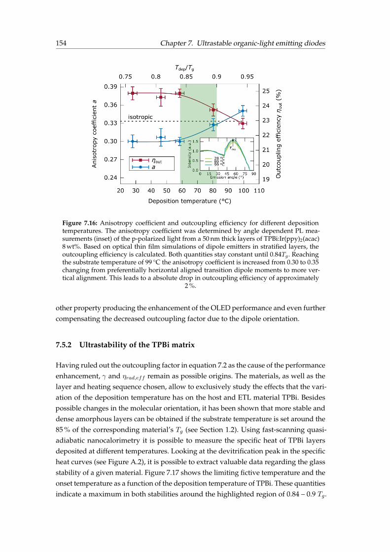
154 Chapter 7. Ultrastable organic-light emitting diodes
Figure 7.16: Anisotropy coefficient and outcoupling efficiency for different depositiontemperatures. The anisotropy coefficient was determined by angle dependent PL mea-surements (inset) of the p-polarized light from a 50 nm thick layers of TPBi:Ir(ppy)2(acac)8 wt%. Based on optical thin film simulations of dipole emitters in stratified layers, theoutcoupling efficiency is calculated. Both quantities stay constant until 0.84Tg. Reachingthe substrate temperature of 99 C the anisotropy coefficient is increased from 0.30 to 0.35changing from preferentially horizontal aligned transition dipole moments to more ver-tical alignment. This leads to a absolute drop in outcoupling efficiency of approximately
2 %.
other property producing the enhancement of the OLED performance and even furthercompensating the decreased outcoupling factor due to the dipole orientation.
7.5.2 Ultrastability of the TPBi matrix
Having ruled out the outcoupling factor in equation 7.2 as the cause of the performanceenhancement, γ and ηrad,eff remain as possible origins. The materials, as well as thelayer and heating sequence chosen, allow to exclusively study the effects that the vari-ation of the deposition temperature has on the host and ETL material TPBi. Besidespossible changes in the molecular orientation, it has been shown that more stable anddense amorphous layers can be obtained if the substrate temperature is set around the85 % of the corresponding material’s Tg (see Section 1.2). Using fast-scanning quasi-adiabatic nanocalorimetry it is possible to measure the specific heat of TPBi layersdeposited at different temperatures. Looking at the devitrification peak in the specificheat curves (see Figure A.2), it is possible to extract valuable data regarding the glassstability of a given material. Figure 7.17 shows the limiting fictive temperature and theonset temperature as a function of the deposition temperature of TPBi. These quantitiesindicate a maximum in both stabilities around the highlighted region of 0.84 – 0.9 Tg.

7.5. Discussion 155
Figure 7.17: Thermal characterization as a function of the deposition temperature of TPBilayers. The fictive temperature (red, left-axis) as a thermal stability parameter and theonset of the glass transition (blue, right-axis) as a kinetic stability parameter of 60 to 80 nmfilms of TPBi as a function of the substrate temperature. These parameters are extractedfrom the heat capacity curves performed using quasi-adiabatic fast-scanning calorimetry,
see Figure A.2 in Appendix A.
Although the T ′f shows a minimum plateau over a wide range between the 20 C and70 C, the kinetic stability shows a clear maximum around 60–70 C, which coincideswith the typical highly stable glass formation range. These results prove that TPBi ispart of the extensive family of organic molecular glass-formers that can be preparedinto their ultrastable glass form when deposited at the optimal Tdep. Although we donot have a direct measure of density changes for TPBi, increased densities have beenobserved for similar OLED materials before [45].
While the absolute changes of the layer density are typically in the range of 1–2 % [45],such subtle difference will likely influence the excitonic properties significantly, as allcouplings and transfer processes come with nanoscale sensitivity [166]. The TPBi layeris the host for the for the green emitter in the G0 devices, in which the 8 wt% doping ofIr(ppy)2(acac) is assumed not to influence the glassy matrix properties decisively. Totest the hypothesis that the changes in stability and molecular packing of the TPBi causethe enhanced efficiencies, the same device architecture is used with three additionalphosphorescent emitters (Ir(MDQ)2(acac), Ir(ppy)3, and FIrpic). Figure 7.13 shows howthe EQE is enhanced when the temperature is set to 66 C for the devices R1, G1 and B1,using the red, the green and the blue emitter respectively. These results further supportthe idea that the host (TPBi) properties are the ones affecting the device performance.

156 Chapter 7. Ultrastable organic-light emitting diodes
The radiative efficiency can be written as the ratio between the radiative decay rate inthe optical cavity (Γ∗r) to the total exciton decay rates [159], which reads
ηrad,eff =Γ∗r
Γ∗r + Γnr= Γ∗rτrad,eff (7.8)
where the Γnr are the nonradiative decay rates. The inverse of the sum of the total exci-ton decay rates is defined as the effective lifetime and can be measured by the photolu-minescence (PL) decay times (see Appendix A). Looking at the increased τrad,eff (i.e. ex-cited state lifetimes of the emitters in the OLED micro cavity) of +15 % (G1), +17 % (R1)and +29 % (B1) in Figure 7.13g,h,i, with the assumption that the radiative rate stays con-stant [159], one can relate the transient time enhancement directly to an improved radia-tive efficiency due to reduced nonradiative rates. The EQE increase can be fully corre-lated to the changes observed for the excited state lifetime τrad,eff . This reduction couldbe rationalized in terms of a possible reduction or suppression of the β-relaxation—molecule vibrations within a cage formed by its neighbors—in the ultrastable glassof TPBi, which could slow down the nonradiative phonon-mediated monomolecularthermal relaxation processes [159]. Similar observations of reduced nonradiative re-combination rates have been observed in polymer-based systems that were preparedin a very rigid form that led to a higher packing density compared to a conventionallyfabricated reference sample [167, 168]. Currently, in vapour-deposited small molecules,a suppression of the β-relaxation has been reported for ultrastable glasses of toluene,n-propanol and 2-picoline by Yu et al. [50] and etoricoxib by Rodríguez-Tinoco et al.[51] but, while caution must be applied at the limited data available, it may be a generalfeature of ultrastable glasses.
However, while the increase of radiative efficiency for the device B1 is significantlylarger with (+29 %), it fails to explain the massive enhancement of the device efficiency(+165 %). In this particular case, host and emitter are energetically in resonance atabout 2.6 eV (see Figure A.3) with respect to their triplet (T1) levels, where a delayedemitter population has been shown [142]. Increased packing would greatly enhancetriplet migration in the film and by that the efficiency. Unfortunately, the transientmeasurements do not allow to investigate this delayed effect in more detail.
The remaining parameter of equation 7.2 determining the OLED EQE is γ. Referringto the heating sequence during device processing, a change in transport properties canonly be expected for the TPBi based layers, because the TCTA hole transport layersundergo identical treatment for all devices. While both j–V characteristics (Figure7.11a and A.1) and EQE vs luminance data (Figure 7.12 and 7.13a, b, c) for the differentdevices look very similar, changes in the mobility may induce subtle changes in theelectron and hole concentration and distribution, which could be a cause for efficiencymodulations. Such carrier transport related changes however do not influence the
7.5. Discussion 157
radiative efficiency ηrad,eff . Hence, with the good agreement of EQE and ηrad,eff fordevices G1 and R1, an altered electrical efficiency can be considered, at first glance,a minor effect. On the contrary, transport changes seem to cause most of the EQEenhancement for the FIrpic based devices B1. Here, it is possible that the resonanttriplet energy character of the TPBi:FIrpic EML as mentioned above is more sensitiveto a re-distribution of the charge carrier and recombination profiles [169].
7.5.3 Other temperature-OLED devices
In reviewing the literature, we only found the work by Mu et al. [151] that addressedthe electroluminescent dependence of a simplified OLED on the deposition tempera-ture of the devices. In their work, they use the simplified stack CBP/CBP:Ir(ppy)3/TPBiprepared under different deposition temperatures (the whole device). While they re-port a significant EQE improvement, it is worth noting that their RT reference deviceonly reached 10.6 % EQE and the best thermally treated OLED 17.9 %, where the latteris about as efficient as the reference in this study (see Table7.2, device G1). Surprisingly,the temperature at which the maximum EQE is reached coincides ours. This effect isattributed by Mu et al. [151] partly to the impact that the deposition temperature hason the surface roughness of the CBP/CBP:Ir(ppy)3 and partly to an enhancement of theelectron and hole mobility of their respective transport layers. However, some crucialdifferences should be pointed out. First, the choice of CBP as HTL and EML with itspoor glass formation ability, the Tg is barely reported in literature due to its difficulty tocreate a CBP glass from the supercooled liquid since it normally crystallises. Secondly,in that work, their best performance is given for the device prepared 7 C above theTg of the CBP, so that it would be a supercooled liquid. This full combination makesharder to decorrelate the impact of each layer properties on device performance.
In another study, performed by Burns et al. [152], the properties of the emissive layer areaddressed in terms of the glass transition. They use a polymer-based OLED preparedby spin coating to study the effect that thermal annealing at different temperatureshas in the device performance. Thermally annealed devices show enhanced perfor-mance (EQE and current efficiencies) compared to the as-prepared sample. Their bestperformance is achieved for the device annealed below the Tg of the emissive layer,whereas a decreasing trend in the performance is seen with increasing the annealingtemperature. Although a clear explanation for the enhancement of the performance ofthe as-prepared device and the annealed below Tg is not provided in their study, wecan reason it in terms of physical ageing and a reduction of the β-relaxation too [167].

158 Chapter 7. Ultrastable organic-light emitting diodes
7.5.4 Lifetime improvement
Besides the EQE, the lifetime of the devices prepared at ∼0.85Tg is also improved (seeFigure 7.14 and Table 7.2). In general, it is a tough and laborious task to investigatethe degradation of OLEDs and correlate these findings to the nanoscopic level of themolecular building blocks [8]. Here, if only a change of the deposition parametersfor EML and ETL (composed mostly of TPBi) lead to a similar correlation with the0.85Tg criteria to form an ultrastable glass, i.e. LT70 peaks at these deposition temper-atures, it can be deduced that the molecular conformation at the nanoscale favours amore durable device operation. A clear correlation between the glass density and thephotostability—which measures the resistance of the material to light irradiation—hasbeen recently established by Qiu et al. [170]. They prepare samples of DO37 (DispersiveOrange 37) glass by physical vapour deposition at different substrates temperaturesand find that glasses prepared at 0.88Tg have, besides higher kinetic stability and higherdensity, higher photostability. They argue that higher density glasses have also higherintermolecular barriers for the molecular rearrangement, which prevent the cis-to-transphotoisomerization causing the loss of photostability in their DO37 glasses. Notwith-standing that some works have reported isomerization reaction of Ir-based emittersdue to the device aging or to thermal heating needed for the vacuum-deposition pro-cess [171], it is still unknown the contribution that isomers—if any—have on the deviceefficiency or degradation [8] mechanism. A qualitative argument for the enhanced sta-bility is like the one used above for increased radiative efficiency. The rigidity of thefilms formed as ultrastable glasses is likely to suppress coupling to generally accessibledecomposition routes present in OLEDs.
7.6 Summary
In summary, this study shows that the performance of state-of-the-art organic light-emitting diodes can be significantly enhanced by optimizing the growth condition ofthe organic layers. We have prepared a highly simplified OLED device and tested itsperformance upon the deposition temperature of its EML and ETL layer, consistingof TPBi. The maximum performance for both the external quantum efficiency and theluminous efficacy, is achieved when the deposition temperature is ca. the 0.85Tg of theTPBi layer, in agreement with the maximum thermal stability.
We have proved that the orientation of the emitter cannot explain this improvementsince it should produce a decrease in the efficiency if solely this factor was considered.We have the same device structure to check for three other emitters, exhibiting all ofthem efficiency enhancements at the∼0.85Tg. We have measured the phosphorescencelifetime in these devices to assess the radiative efficiency of the emission layer. The
7.6. Summary 159
results have shown that the enhancements in devices’ EQE can be well-correlated toan increased radiative efficiency which, in turn, exhibit an excellent correlation withthe thermal stability of the TPBi layer. We rationalize these findings with a likely de-crease of the β-relaxation in the TPBi ultrastable matrix which would decrease thenonradiative decay processes.
A good correlation has also been found for the improvement of the OLED’s lifetimeand the ∼0.85Tg deposition temperature. A better packing and rigidity of the matrix isalso thought to preclude some of the degradation routes of the emitters and, therefore,increasing the operational lifetime.

Chapter 8
Conclusions
The main goal of this work was to deepen into the understanding of the glass transitionphenomenon through organic vapour-deposited glasses. For that, we have exploredand characterised several facets of vapour-deposited glasses of different molecularglass-formers, addressing both fundamental aspects as well as their possible applica-tion in organic light-emitting diode technology. As materials, we have first chosentoluene, a model glass-former which ultrastability had been previously established.The other materials used are organic semiconductor molecules widely employed in theorganic electronics field.
An extensive part of the results presented in this work has been obtained using quasi-adiabatic fast-scanning nanocalorimetry. Various key features make nanocalorimetrya prominent technique to assess several aspects of organic vapour-deposited glasses.First, it allows measuring in situ the as deposited samples with the possibility to cleanthe devices just after the measurement of each sample. Second, the high heating ratespush the devitrification process to much higher temperature ranges where other—moreconventional—techniques do not have access. Third, the sensitivity of the techniqueallows sensing the heat capacity of very low masses, as in the case of nanometric films.
Glasses of toluene, TPD, α-NPD, TCTA and TPBi have been deposited using physicalvapour deposition in a broad range of deposition temperatures at low growth ratesof ≈0.2 nm s−1. The deposition temperature has been shown to play a significant rolein setting the kinetic and thermodynamic stability of glasses of all the studied ma-terials. Glasses prepared at deposition temperatures around 0.85-0.89Tg exhibit themaximum stability. Glasses prepared above this maximum exhibit a limiting fictivetemperature equal to the deposition temperature, which would indicate equilibrationbetween glassy and liquid states. Specifically, for toluene, TPD and α-NPD, we haveseen that the thermodynamic stability is independent of the thickness of the samplefor the deposition temperatures and thickness range addressed. These results are inagreement with previous findings corresponding to other molecular glass-formingsystems.
162 Chapter 8. Conclusions
We have seen how vapour-deposited glasses transform into the supercooled liquid viaa propagating growth front depending on their Tdep, in stark contrast to conventionalglasses prepared from the liquid. The transformation mechanism has been inferredfrom the calorimetric trace of the devitrification using an ad hoc normalisation pro-cedure. As has been demonstrated for other organic molecules, in toluene, the prop-agation velocity of this transformation front is firmly dominated by the mobility ofthe supercooled liquid molecules. A linear relation holds between the logarithm of thefront velocity and the logarithm of the relaxation time of the liquid for an extendedtemperature range, covering eight orders of magnitude. For TPD, different activationenergies are obtained at low and high temperature when considering an Arrheniusdependence, which is consistent the observed relation between front velocity and themobility of the supercooled liquid layer.
As seen for toluene, TPD and α-NPD, the most thermodynamically stable glassespresent the slowest transformation rates and higher crossover lengths. In the caseof toluene, the stability of the glass and the mobility of the liquid seems enough todetermine the growth front velocity. On the other hand, in both organic semiconductorglass-formers, the stability does not univocally determine the front velocity and theorientation of the molecules—which also depends on the Tdep—is proposed to be alsoone of the factors governing the assimilation of the molecules from the glass into thesupercooled liquid front. Our study suggests a prominent relation between moleculargeometry, and therefore anisotropy of the produced glass, and transformation veloc-ity. In that scenario, the one-to-one relationship between growth front velocity andstability of toluene would suggest a much lower degree, if any, of molecular orienta-tion. It would be interesting to reproduce similar studies of growth front velocity onwell-known isotropic systems.
Together with the front velocity, we have also seen how the extend into which the het-erogenous mechanism dominates strongly depends on the Tdep. In glasses depositedclose to Tg , the bulk transformation rapidly dominates within the very first nanometersof front transformation. Surprisingly, the vgr − T ′f good correlation in toluene systemis not reproduced for the crossover length. We have seen up to a 4-fold change in thecrossover length of glasses with the same thermal stability but prepared at differentdeposition temperatures. A possible explanation for this behaviour could be the exis-tence of two distinct mechanisms of glass formation at temperatures close and far fromTg . A thorough analysis of the homogeneous (bulk) glass transition in an extensivedeposition temperature range would be necessary to confirm or refute this hypothesisin the toluene system. On the other hand, the crossover length of TPD and a-NPDglasses of same T ′f but deposited at different Tdep—above and below Tg—is expectedto be distinct since they already present significantly different growth front velocities.
To gain access to the bulk transformation, we have capped TPD layers with a higher-Tg
Chapter 8. Conclusions 163
material—TCTA—and have measured its devitrification also using nanocalorimetry.The growth transformation front of TPD films is effectively suppressed when the highmobility interface is capped, and then the glass transition occurs via a bulk mechanism.These results agree with previous results on the IMC/TNB system and the kineticfacilitation framework. We have successfully capped glasses from a wide range ofstabilities. By testing different multilayer configurations, we have been able to inferthat there is only one growth front mechanism starting from the free surface and nonein the organic/substrate interface, regardless the stability of the glass.
The suppression (or significant delay) of the high-mobility layer improves the isother-mal stability of ultrastable glasses. Further experiments, though, are required to fullyexplore the mechanisms behind the rejuvenation of the ultrastable—and also lessstable—glasses. Capped organic layers conform the core of OLEDs, where the im-proved isothermal stability could play a role in determining the maximum workingtemperature.
We have used the newly implemented 3ω–Völklein method in GNaM to measure—insitu—the thermal conductivity in organic vapour-deposited glasses. First, we haveused this technique to monitor the growth of a film from the very first stages. Thesensitivity of the technique has allowed us to identify different growth regimes of thefilm before becoming continuous. We have started to explored the possibility to usethis strategy to obtain valuable information on the different growth mechanisms ofvapour-deposited glasses at various Tdep.
Secondly, we have shown that the in-plane thermal conductivity of TPD and α-NPDvapour-deposited can be controlled by the deposition temperature and that it corre-lates well with the reported anisotropy data. Using the well-established 3ω, we havebeen able to establish a thermal anisotropy ratio of ≈37 % for TPD between in-planeand out-of-plane thermal conductivities. Complementary molecular dynamics simu-lations have shown how the thermal conductivity is favoured along the direction ofthe backbone of the TPD molecule and, with a simplified model, how this can explainthe anisotropy in thermal conductivity even in such small molecule systems. The ther-mal transport anisotropy is at odds with electronic transport that favours propagationalong the perpendicular direction to the long axis of the molecule provided there issufficient π-π interaction. This strategy could be employed in future developments toimplement small molecule thin films for its use in thermoelectric-based applications.
We have prepared a proof-of-concept OLED device to test the impact of highly stableglasses in a real state-of-the-art applicaton. We have demonstrated that a significantenhancement of the efficiency and lifetime of a simplified OLED stack correlates withthe increased stability and better packing of the electron and host transport layerswhen deposited at temperatures in the vicinity of 0.85Tg. At this same depositiontemperature, an increase of the emitter’s excited state lifetime is also observed. We
164 Chapter 8. Conclusions
have rationalised this improvement with a decrease of the nonradiative recombinationrates due to a better packed and more rigid environment. Regarding the lifetime of thedevices, the rigidity of the matrix is also likely to suppress or slow down the accessibledecomposition routes present in OLED devices. While the orientation of the emitter hasbeen completely ruled out as a possible factor influencing the efficiency, other factors,such as the charge transport properties are not readily discarded to play also a minorrole. Further work needs to be done to understand better and quantify the contributionof the several factors implied in a device performance.
We anticipate that our findings can be generalised to any OLED, leading to improve-ments in both efficiency and lifetime, especially because they can be directly correlatedto a very fundamental material’s property such as the glass transition temperature.Therefore, the present study provides an additional approach to existing strategies—material development and advanced optical solutions—for efficiency optimisation.
Finally, we would like to remark the significance that the findings from this studyprovide both in the fundamental understanding of vapour-deposited glasses and theirpotential applications for state-of-the-art technologies.

Appendix A
Supplementary information
In this appendix, we briefly describe two of the techniques that have been used inChapter 7 to quantify the photoluminescence lifetime of the emission layer of the R1,G1 and B1 devices and the orientation of the emitter for the device G0 as a functionof the deposition temperature. These measurements are framed in the context of theongoing collaboration with the group of Prof. Dr Sebastian Reineke from the IAPP. Thetime-resolved experiments were carried out by Paul-Anton Will. The angular resolvedphotoluminescence spectra were measured by the author whereas the modelling andthe development of the fitting algorithm to extract the anisotropy value were carriedout by Christian Hänisch. Moreover, we include some supplementary figures that havebeen left out of the main text for clarity purposed.
A.1 Time-resolved photoluminescence
For measuring the time-resolved photoluminescence, the OLEDs R1, G1, B1 were ex-cited with a pulsed nitrogen laser (MNL 202-C/ATM 200, Lasertechnik Berlin) with anoperational wavelength of 337.1 nm. A mask was used to ensure excitation to be onlyin the active area of the devices. The emitted light is focused and recorded with a Siamplified photodetector (PDA100A-EC, Thorlabs). Various long pass filters are usedto exclude the laser and fluorescence from the signal.
A.2 Orientation of the emitter measurements
The anisotropy coefficient as a measure of the emitter molecules’ transition dipolemoments is extracted from angular resolved photoluminescence spectra following themethod of Frischeisen et al. [165]. We use a 50 nm thick encapsulated single layer ofTPBi:Ir(ppy)2(acac) evaporated on a 1.1 mm thick Eagle XG glass (Corning) substratewhich is attached to a 4 cm glass half-cylinder prism via index matching oil. The organicfilm is excited optically by a 405 nm laser diode (STAR405F10, Roithner Lasertechnik).
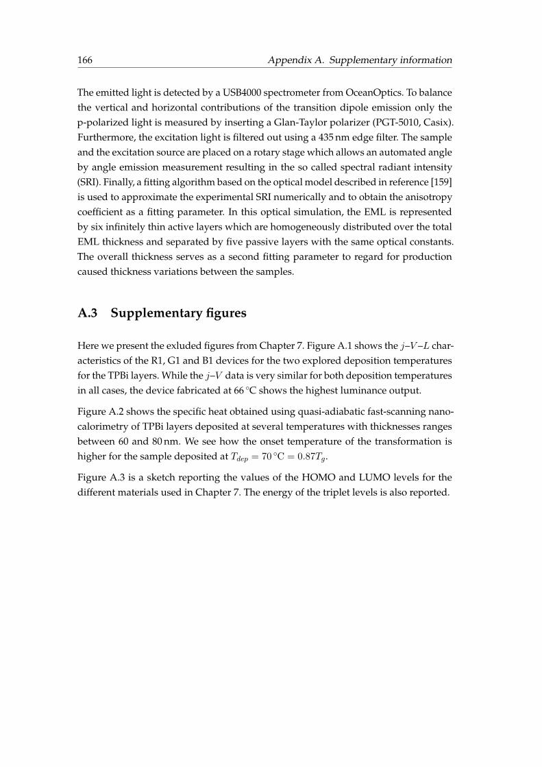
166 Appendix A. Supplementary information
The emitted light is detected by a USB4000 spectrometer from OceanOptics. To balancethe vertical and horizontal contributions of the transition dipole emission only thep-polarized light is measured by inserting a Glan-Taylor polarizer (PGT-5010, Casix).Furthermore, the excitation light is filtered out using a 435 nm edge filter. The sampleand the excitation source are placed on a rotary stage which allows an automated angleby angle emission measurement resulting in the so called spectral radiant intensity(SRI). Finally, a fitting algorithm based on the optical model described in reference [159]is used to approximate the experimental SRI numerically and to obtain the anisotropycoefficient as a fitting parameter. In this optical simulation, the EML is representedby six infinitely thin active layers which are homogeneously distributed over the totalEML thickness and separated by five passive layers with the same optical constants.The overall thickness serves as a second fitting parameter to regard for productioncaused thickness variations between the samples.
A.3 Supplementary figures
Here we present the exluded figures from Chapter 7. Figure A.1 shows the j–V –L char-acteristics of the R1, G1 and B1 devices for the two explored deposition temperaturesfor the TPBi layers. While the j–V data is very similar for both deposition temperaturesin all cases, the device fabricated at 66 C shows the highest luminance output.
Figure A.2 shows the specific heat obtained using quasi-adiabatic fast-scanning nano-calorimetry of TPBi layers deposited at several temperatures with thicknesses rangesbetween 60 and 80 nm. We see how the onset temperature of the transformation ishigher for the sample deposited at Tdep = 70 C = 0.87Tg.
Figure A.3 is a sketch reporting the values of the HOMO and LUMO levels for thedifferent materials used in Chapter 7. The energy of the triplet levels is also reported.
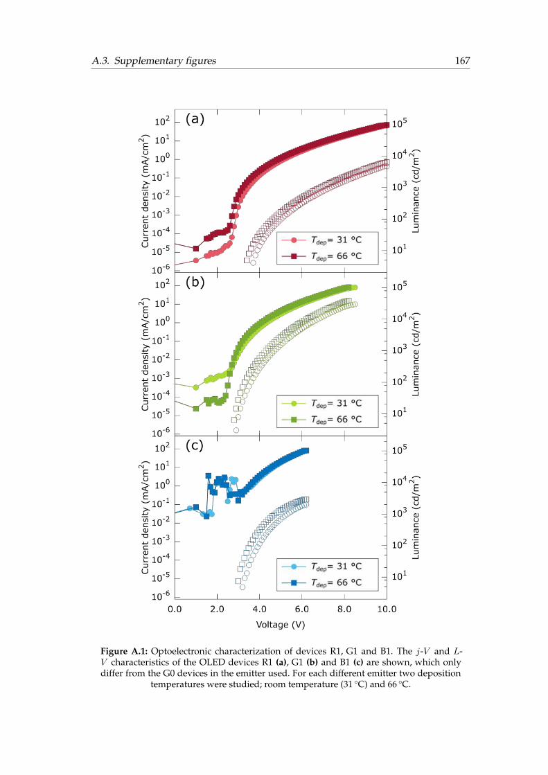
A.3. Supplementary figures 167
Figure A.1: Optoelectronic characterization of devices R1, G1 and B1. The j-V and L-V characteristics of the OLED devices R1 (a), G1 (b) and B1 (c) are shown, which onlydiffer from the G0 devices in the emitter used. For each different emitter two deposition
temperatures were studied; room temperature (31 C) and 66 C.
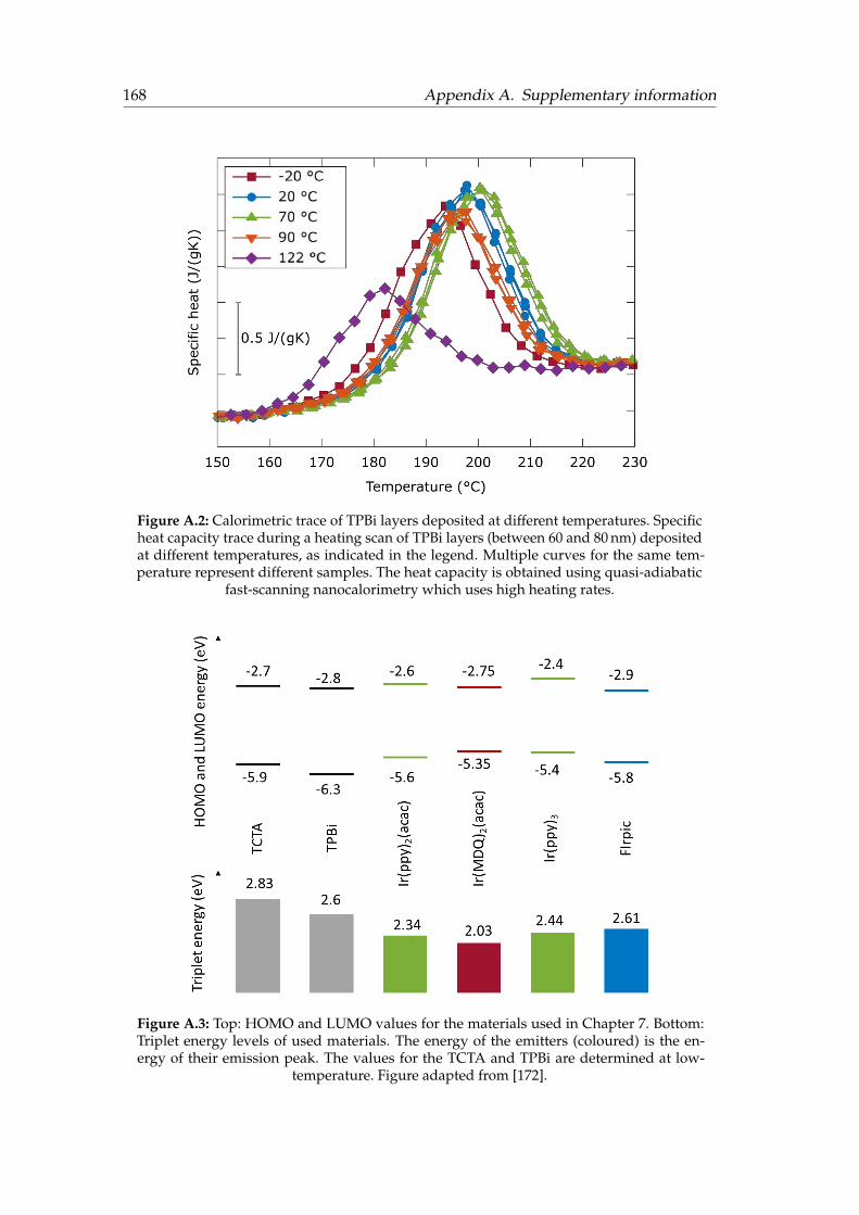
168 Appendix A. Supplementary information
Figure A.2: Calorimetric trace of TPBi layers deposited at different temperatures. Specificheat capacity trace during a heating scan of TPBi layers (between 60 and 80 nm) depositedat different temperatures, as indicated in the legend. Multiple curves for the same tem-perature represent different samples. The heat capacity is obtained using quasi-adiabatic
fast-scanning nanocalorimetry which uses high heating rates.
Figure A.3: Top: HOMO and LUMO values for the materials used in Chapter 7. Bottom:Triplet energy levels of used materials. The energy of the emitters (coloured) is the en-ergy of their emission peak. The values for the TCTA and TPBi are determined at low-
temperature. Figure adapted from [172].

169
References
[1] Pablo G. Debenedetti and Frank H. Stillinger. “Supercooled liquids and theglass transition”. In: Nature 410.6825 (Mar. 2001), pp. 259–267. D O I: 10.1038/35065704. arXiv: 9911023v1 [arXiv:cond-mat].
[2] A. L. Greer. “Metallic Glasses”. In: Science 267.5206 (Mar. 1995), pp. 1947–1953.D O I: 10.1126/science.267.5206.1947.
[3] Ian L. Pegg. “Turning nuclear waste into glass”. In: Physics Today 68.2 (Feb.2015), pp. 33–39. D O I: 10.1063/PT.3.2687.
[4] Gregory M. Fahy et al. “Physical and biological aspects of renal vitrification”.In: Organogenesis 5.3 (July 2009), pp. 167–175. D O I: 10.4161/org.5.3.9974.
[5] John W. Delano. “Pristine lunar glasses: Criteria, data, and implications”. In:Journal of Geophysical Research: Solid Earth 91.B4 (Mar. 1986), pp. 201–213. D O I:10.1029/JB091iB04p0D201.
[6] Bruno C. Hancock and George Zografi. “Characteristics and Significance ofthe Amorphous State in Pharmaceutical Systems”. In: Journal of PharmaceuticalSciences 86.1 (Jan. 1997), pp. 1–12. D O I: 10.1021/js9601896.
[7] Bernard Geffroy, Philippe le Roy, and Christophe Prat. “Organic light-emittingdiode (OLED) technology: materials, devices and display technologies”. In:Polymer International 55.6 (June 2006), pp. 572–582. D O I: 10.1002/pi.1974.
[8] Sebastian Scholz et al. “Degradation Mechanisms and Reactions in OrganicLight-Emitting Devices”. In: Chemical Reviews 115.16 (Aug. 2015), pp. 8449–8503.D O I: 10.1021/cr400704v.
[9] Salvatore Torquato. “Glass transition: hard knock for thermodynamics”. In:Nature 405.6786 (June 2000), pp. 521–523. D O I: 10.1038/35014711.
[10] S. F. Swallen et al. “Organic Glasses with Exceptional Thermodynamic andKinetic Stability”. In: Science 315.5810 (Jan. 2007), pp. 353–356. D O I: 10.1126/science.1135795.
[11] Andrea Cavagna. “Supercooled liquids for pedestrians”. In: Physics Reports476.4-6 (June 2009), pp. 51–124. D O I: 10.1016/j.physrep.2009.03.003.
[12] C. M. Roland. “Characteristic relaxation times and their invariance to thermo-dynamic conditions”. In: Soft Matter 4.12 (Nov. 2008), p. 2316. D O I: 10.1039/b804794d.

170 REFERENCES
[13] CA Austen Angell. “Formation of Glasses from Liquids and Biopolymers”. In:Science 267.5206 (Mar. 1995), pp. 1924–1935. D O I: 10.1126/science.267.5206.1924.
[14] Mark D. Ediger. “Spatially heterogeneous dynamics in supercooled liquids”. In:Annual review of physical chemistry 51.1 (Oct. 2000), pp. 99–128. D O I: 10.1146/annurev.physchem.51.1.99. arXiv: 0066-426X.
[15] E. Vidal Russell and N. E. Israeloff. “No Title”. In: Nature 408.6813 (Dec. 2000),pp. 695–698. D O I: 10.1038/35047037.
[16] Donna Perera and Peter Harrowell. “Consequences of kinetic inhomogeneitiesin glasses”. In: Physical Review E 54.2 (Aug. 1996), pp. 1652–1662. D O I: 10.1103/PhysRevE.54.1652.
[17] Peter G Wolynes. “Spatiotemporal structures in aging and rejuvenating glasses”.In: Proceedings of the National Academy of Sciences of the United States of America106.5 (Feb. 2009), pp. 1353–8. D O I: 10.1073/pnas.0812418106.
[18] Marcus T. Cicerone and Mark D. Ediger. “Enhanced translation of probe moleculesin supercooled o-terphenyl: Signature of spatially heterogeneous dynamics?”In: The Journal of Chemical Physics 104.18 (May 1996), pp. 7210–7218. D O I : 10.1063/1.471433.
[19] AP Sokolov et al. “Dynamics of strong and fragile glass formers: Differences andcorrelation with low-temperature properties”. In: Physical review letters 71.13(1993), pp. 1–4.
[20] Gregory B. McKenna. “Physical Aging in Glasses and Composites”. In: Long-Term Durability of Polymeric Matrix Composites. Ed. by Kishore V. Pochiraju,Gyaneshwar P. Tandon, and Gregory A. Schoeppner. Vol. 44. 8. Boston, MA:Springer US, Nov. 2012, pp. 237–309. D O I: 10.1007/978-1-4419-9308-3_7. arXiv: 1011.1669.
[21] Cornelius T. Moynihan et al. “Dependence of the Fictive Temperature of Glasson Cooling Rate”. In: Journal of the American Ceramic Society 59.1-2 (Jan. 1976),pp. 12–16. D O I: 10.1111/j.1151-2916.1976.tb09376.x.
[22] M. G. Abiad, M. T. Carvajal, and O. H. Campanella. “A Review on Methods andTheories to Describe the Glass Transition Phenomenon: Applications in Foodand Pharmaceutical Products”. In: Food Engineering Reviews 1.2 (Dec. 2009),pp. 105–132. D O I: 10.1007/s12393-009-9009-1.
[23] Hideaki Hikawa, Masaharu Oguni, and Hiroshi Suga. “Construction of an adi-abatic calorimeter for a vapor-deposited sample and thermal characterizationof amorphous butyronitrile”. In: Journal of Non-Crystalline Solids 101.1 (1988),pp. 90–100. D O I: 10.1016/0022-3093(88)90373-0.
[24] K Takeda, O Yamamuro, and Hiroshi Suga. “Calorimetric study on structuralrelaxation of 1-pentene in vapor deposited and liquid-quenched glassy states”.In: The Journal of Physical Chemistry 99 (1995), pp. 1602–1607.
REFERENCES 171
[25] Christopher J Ellison and John M Torkelson. “The distribution of glass-transitiontemperatures in nanoscopically confined glass formers”. In: Nature Materials2.10 (Sept. 2003), pp. 695–700. D O I: 10.1038/nmat980.
[26] C. R. Daley et al. “Comparing surface and bulk flow of a molecular glass for-mer”. In: Soft Matter 8.7 (2012), p. 2206. D O I: 10.1039/c2sm06826e.
[27] L. Zhu et al. “Surface Self-Diffusion of an Organic Glass”. In: Physical ReviewLetters 106.25 (June 2011), p. 256103. D O I: 10.1103/PhysRevLett.106.256103.
[28] Kenneth L. Kearns, S. F. Swallen, and Mark D. Ediger. “Hiking down the energylandscape: Progress toward the Kauzmann temperature via vapor deposition”.In: The Journal of Physical Chemistry B 112.16 (Apr. 2008), pp. 4934–4942. D O I:10.1021/jp7113384.
[29] Edgar Leon-Gutierrez et al. “Stability of thin film glasses of toluene and ethyl-benzene formed by vapor deposition: an in situ nanocalorimetric study”. In:Phys. Chem. Chem. Phys. 12.44 (Nov. 2010), pp. 14693–14698. D O I : 10.1039/C0CP00208A.
[30] Edgar Leon-Gutierrez et al. “Correction: Stability of thin film glasses of tolueneand ethylbenzene formed by vapor deposition: an in situ nanocalorimetricstudy”. In: Phys. Chem. Chem. Phys. 18.11 (2016), pp. 8244–8245. D O I: 10.1039/C6CP90023B.
[31] K. L. Ngai, Li-Min Wang, and Hai-Bin Yu. “Relating Ultrastable Glass Forma-tion to Enhanced Surface Diffusion via the Johari-Goldstein β-Relaxation inMolecular Glasses”. In: The Journal of Physical Chemistry Letters 8.12 (June 2017),pp. 2739–2744. D O I: 10.1021/acs.jpclett.7b01192.
[32] Zahra Fakhraai. “The Role of Surface-Mediated Equilibration in the Forma-tion of Stable Glasses”. 8th International Discussion Meeting on Relaxations inComplex Systems. 2017.
[33] Cristian Rodríguez-Tinoco et al. “Highly stable glasses of celecoxib: Influenceon thermo-kinetic properties, microstructure and response towards crystal growth”.In: Journal of Non-Crystalline Solids 0 (Aug. 2014), pp. –. D O I : 10.1016/j.jnoncrysol.2014.07.031.
[34] Cristian Rodríguez-Tinoco et al. “Evaluation of Growth Front Velocity in Ul-trastable Glasses of Indomethacin over a Wide Temperature Interval”. In: TheJournal of Physical Chemistry B 118.36 (Sept. 2014), pp. 10795–10801. D O I : 10.1021/jp506782d.
[35] Mathias Ahrenberg et al. “In situ investigation of vapor-deposited glasses oftoluene and ethylbenzene via alternating current chip-nanocalorimetry”. In:The Journal of Chemical Physics 138.2 (Jan. 2013), p. 024501. D O I: 10.1063/1.4773354.
172 REFERENCES
[36] Kenneth L. Kearns et al. “Observation of low heat capacities for vapor-depositedglasses of indomethacin as determined by AC nanocalorimetry”. In: The Journalof Chemical Physics 133.1 (July 2010), p. 014702. D O I: 10.1063/1.3442416.
[37] Z Chen et al. “Dynamics of glass-forming liquids. XVI. Observation of ultra-stable glass transformation via dielectric spectroscopy”. In: The Journal of Chem-ical Physics 138.12 (Mar. 2013), 12A519. D O I: 10.1063/1.4771695.
[38] A. Sepúlveda et al. “Role of Fragility in the Formation of Highly Stable OrganicGlasses”. In: Physical Review Letters 113.4 (July 2014), p. 045901. D O I: 10.1103/PhysRevLett.113.045901.
[39] Shakeel S. Dalal, Zahra Fakhraai, and Mark D. Ediger. “High-Throughput El-lipsometric Characterization of Vapor-Deposited Indomethacin Glasses”. In:The Journal of Physical Chemistry B 117.49 (Dec. 2013), pp. 15415–15425. D O I:10.1021/jp405005n.
[40] Diane M. Walters, Ranko Richert, and Mark D. Ediger. “Thermal stability ofvapor-deposited stable glasses of an organic semiconductor”. In: The Journal ofChemical Physics 142.13 (Apr. 2015), p. 134504. D O I: 10.1063/1.4916649.
[41] A. Sepúlveda et al. “Stable glasses of indomethacin andα,α,β-tris-naphthylbenzenetransform into ordinary supercooled liquids”. In: The Journal of Chemical Physics137.20 (Nov. 2012), p. 204508. D O I: 10.1063/1.4768168.
[42] Stephen F. Swallen et al. “Stable Glass Transformation to Supercooled Liquidvia Surface-Initiated Growth Front”. In: Physical Review Letters 102.6 (Feb. 2009),p. 065503. D O I: 10.1103/PhysRevLett.102.065503.
[43] R. Scott Smith, R. Alan May, and Bruce D. Kay. “Probing Toluene and Ethyl-benzene Stable Glass Formation Using Inert Gas Permeation”. In: The Journal ofPhysical Chemistry Letters 6.18 (Sept. 2015), pp. 3639–3644. D O I: 10.1021/acs.jpclett.5b01611.
[44] Shakeel S. Dalal et al. “Density and birefringence of a highly stable α,α,β-trisnaphthylbenzene glass”. In: The Journal of chemical physics 136.20 (May 2012),p. 204501. D O I: 10.1063/1.4719532.
[45] Shakeel S. Dalal et al. “Tunable molecular orientation and elevated thermal sta-bility of vapor-deposited organic semiconductors”. In: Proceedings of the NationalAcademy of Sciences 112.14 (Apr. 2015), pp. 4227–4232. D O I: 10.1073/pnas.1421042112.
[46] Kikujiro Ishii et al. “Behavior of glass and supercooled liquid Alkylbenzenesvapor-deposited on cold substrates: Toward the understanding of the curiouslight scattering observed in some supercooled liquid states”. In: Bulletin of theChemical Society of Japan 82.10 (2009), pp. 1240–1247. D O I: 10.1246/bcsj.82.1240.
REFERENCES 173
[47] Kenneth L. Kearns et al. “High Modulus Organic Glasses Prepared by PhysicalVapor Deposition”. In: Advanced Materials 22.1 (Jan. 2010), pp. 39–42. D O I: 10.1002/adma.200901673.
[48] Jessica M. Torres et al. “Substrate Temperature to Control Moduli and Wa-ter Uptake in Thin Films of Vapor Deposited <i>N,N</i> ’-Di(1-naphthyl)-<i>N,N</i> ’-diphenyl-(1,1’-biphenyl)-4,4’-diamine (NPD)”. In: The Journal ofPhysical Chemistry B 119.35 (2015), pp. 11928–11934. D O I: 10.1021/acs.jpcb.5b05814.
[49] Kevin J Dawson et al. “Highly stable indomethacin glasses resist uptake ofwater vapor”. In: The journal of physical chemistry. B 113.8 (Feb. 2009), pp. 2422–7.D O I: 10.1021/jp808838t.
[50] H. B. Yu et al. “Suppression of β Relaxation in Vapor-Deposited UltrastableGlasses”. In: Physical review letters 115.18 (Oct. 2015), p. 185501. D O I: 10.1103/PhysRevLett.115.185501.
[51] Cristian Rodríguez-Tinoco et al. “Secondary relaxation in ultrastable etoricoxib:evidence of correlation with structural relaxation”. In: to be determined (2017).Forthcoming.
[52] Ankit Gujral et al. “Structural Characterization of Vapor-Deposited Glasses ofan Organic Hole Transport Material with X-ray Scattering”. In: Chemistry ofMaterials 27.9 (May 2015), pp. 3341–3348. D O I: 10.1021/acs.chemmater.5b00583.
[53] Deepanjan Bhattacharya and Vlad Sadtchenko. “Enthalpy and high tempera-ture relaxation kinetics of stable vapor-deposited glasses of toluene”. In: TheJournal of Chemical Physics 141.9 (Sept. 2014), p. 094502. D O I: 10.1063/1.4893716.
[54] Cristian Rodríguez-Tinoco et al. “Transformation kinetics of vapor-depositedthin film organic glasses: the role of stability and molecular packing anisotropy”.In: Phys. Chem. Chem. Phys. 17.46 (Dec. 2015), pp. 31195–31201. D O I: 10.1039/C5CP04692K. arXiv: arXiv:1011.1669v3.
[55] Tomás Pérez-Castañeda et al. “Suppression of tunneling two-level systems inultrastable glasses of indomethacin”. In: Proceedings of the National Academy ofSciences of the United States of America (July 2014), pp. 1–6. D O I: 10.1073/pnas.1405545111.
[56] Sergio Luis L M Ramos et al. “Character of Devitrification, Viewed from En-thalpic Paths, of the Vapor-Deposited Ethylbenzene Glasses”. In: The Journalof Physical Chemistry B 115.49 (Dec. 2011), pp. 14327–14332. D O I : 10.1021/jp203612s.
[57] Lei Zhu and Lian Yu. “Generality of forming stable organic glasses by vapordeposition”. In: Chemical Physics Letters 499.1-3 (Oct. 2010), pp. 62–65. D O I:10.1016/j.cplett.2010.09.010.
174 REFERENCES
[58] Katherine R. Whitaker et al. “Highly Stable Glasses of cis -Decalin and cis /trans -Decalin Mixtures”. In: The Journal of Physical Chemistry B 117.42 (Oct.2013), pp. 12724–12733. D O I: 10.1021/jp400960g.
[59] Katherine R. Whitaker et al. “Kinetic stability and heat capacity of vapor-depositedglasses of o -terphenyl”. In: The Journal of Chemical Physics 143.8 (Aug. 2015),p. 084511. D O I: 10.1063/1.4929511.
[60] Y. Z. Chua et al. “Glass transition and stable glass formation of tetrachloromethane”.In: The Journal of Chemical Physics 144.24 (June 2016), p. 244503. D O I: 10.1063/1.4954665.
[61] Hai-Bin Yu, Yuansu Luo, and Konrad Samwer. “Ultrastable Metallic Glass”. In:Advanced Materials 25.41 (Nov. 2013), pp. 5904–5908. D O I : 10.1002/adma.201302700.
[62] Heedong Yoon et al. “An Ultrastable Polymeric Glass: Amorphous Fluoropoly-mer with Extreme Fictive Temperature Reduction by Vacuum Pyrolysis”. In:Macromolecules 50.11 (June 2017), pp. 4562–4574. D O I: 10.1021/acs.macromol.7b00623.
[63] Sébastien Léonard and Peter Harrowell. “Macroscopic facilitation of glassy re-laxation kinetics: Ultrastable glass films with frontlike thermal response”. In:The Journal of chemical physics 133.24 (Dec. 2010), p. 244502. D O I: 10.1063/1.3511721.
[64] Ricardo Gutiérrez and Juan P Garrahan. “Front propagation versus bulk relax-ation in the annealing dynamics of a kinetically constrained model of ultrastableglasses”. In: Journal of Statistical Mechanics: Theory and Experiment 2016.7 (July2016), p. 074005. D O I : 10.1088/1742-5468/2016/07/074005. arXiv:1604.03495.
[65] Sadanand Singh, Mark D. Ediger, and JJ de Pablo. “Ultrastable glasses from insilico vapour deposition”. In: Nature materials 12.2 (Feb. 2013), pp. 139–44. D O I:10.1038/nmat3521.
[66] Glen M Hocky, Ludovic Berthier, and David R Reichman. “Equilibrium ultra-stable glasses produced by random pinning”. In: The Journal of chemical physics141.22 (Dec. 2014), p. 224503. D O I: 10.1063/1.4903200.
[67] Ludovic Berthier et al. “Equilibrium Sampling of Hard Spheres up to the Jam-ming Density and beyond”. In: Physical Review Letters 116.23 (June 2016), p. 238002.D O I: 10.1103/PhysRevLett.116.238002. arXiv: 1511.06182.
[68] C. Austen Angell. “Fragile Glass Formers: Evidence for a New Paradigm, anda New Relation to Strong Liquids”. In: Structural Glasses and Supercooled Liquids:Theory, Experiment, and Applications. Hoboken, NJ, USA: John Wiley & Sons, Inc.,Mar. 2012, pp. 237–278. D O I: 10.1002/9781118202470.ch7.
[69] Y. Z. Chua et al. “How much time is needed to form a kinetically stable glass?AC calorimetric study of vapor-deposited glasses of ethylcyclohexane”. In: The

REFERENCES 175
Journal of Chemical Physics 142.5 (Feb. 2015), p. 054506. D O I: 10.1063/1.4906806.
[70] Donald M. Mattox. “Introduction”. In: Handbook of Physical Vapor Deposition(PVD) Processing. Elsevier, 2010, pp. 1–24. D O I : 10.1016/B978-0-8155-2037-5.00001-0.
[71] Donald M. Mattox. “The “Good” Vacuum (Low Pressure) Processing Environ-ment”. In: Handbook of Physical Vapor Deposition (PVD) Processing. Elsevier, 2010,pp. 73–145. D O I: 10.1016/B978-0-8155-2037-5.00003-4.
[72] Osamu Yamamuro et al. “Calorimetric Study of Glassy and Liquid Toluene andEthylbenzene: Thermodynamic Approach to Spatial Heterogeneity in Glass-Forming Molecular Liquids”. In: The Journal of Physical Chemistry B 102.9 (Feb.1998), pp. 1605–1609. D O I: 10.1021/jp973439v.
[73] Hai-Feng Xiang et al. “Method for measurement of the density of thin filmsof small organic molecules”. In: The Review of scientific instruments 78.3 (2007),p. 034104. D O I: 10.1063/1.2712932.
[74] Terry M. Tritt. Thermal conductivity : theory, properties, and applications. KluwerAcademic/Plenum Publishers, 2004, p. 290.
[75] M.Yu. Efremov et al. “Thin-film differential scanning nanocalorimetry: heatcapacity analysis”. In: Thermochimica Acta 412.1-2 (Mar. 2004), pp. 13–23. D O I:10.1016/j.tca.2003.08.019.
[76] Aitor Fernandez Lopeandia et al. “Heat transfer in symmetric U-shaped mi-croreactors for thin film calorimetry”. In: Journal of Micromechanics and Microengi-neering 16.5 (May 2006), pp. 965–971. D O I: 10.1088/0960-1317/16/5/013.
[77] J. Rodríguez-Viejo and A. F. Lopeandía. “Quasi-adiabatic, Membrane-Based,Highly Sensitive Fast Scanning Nanocalorimetry”. In: Fast Scanning Calorimetry.Cham: Springer International Publishing, 2016, pp. 105–149. D O I : 10.1007/978-3-319-31329-0_3.
[78] Manel Molina-Ruiz. “Nanocalorimetric studies of size effects in magnetic ox-ides and formation kinetics in silicides”. PhD thesis. Universitat Autònoma deBarcelona, 2014.
[79] Aitor Fernandez Lopeandia. “Development of Membrane-based Calorimetersto Measure Phase Transitions at the Nanoscale”. PhD thesis. Universitat Autònomade Barcelona, 2007, p. 205.
[80] David G. Cahill. “Thermal conductivity measurement from 30 to 750 K: The 3ωmethod”. In: Review of Scientific Instruments 61.2 (Feb. 1990), pp. 802–808. D O I:10.1063/1.1141498. arXiv: arXiv:1011.1669v3.
[81] David G. Cahill, M. Katiyar, and J. R. Abelson. “Thermal conductivity of a-Si:H thin films”. In: Physical Review B 50.9 (Sept. 1994), pp. 6077–6081. D O I:10.1103/PhysRevB.50.6077.
176 REFERENCES
[82] Tao Tong and Arun Majumdar. “Reexamining the 3-omega technique for thinfilm thermal characterization”. In: Review of Scientific Instruments. Vol. 77. 10.American Institute of Physics, Oct. 2006, p. 104902. D O I: 10.1063/1.2349601.
[83] F. Volklein and T. Starz. “Thermal conductivity of thin films-experimental meth-ods and theoretical interpretation”. In: XVI ICT ’97. Proceedings ICT’97. 16th In-ternational Conference on Thermoelectrics (Cat. No.97TH8291). IEEE, 1997, pp. 711–718. D O I: 10.1109/ICT.1997.667630.
[84] A. Sikora et al. “Highly sensitive thermal conductivity measurements of sus-pended membranes (SiN and diamond) using a 3ω-Völklein method”. In: Re-view of Scientific Instruments 83.5 (May 2012), p. 054902. D O I: 10.1063/1.4704086. arXiv: 1201.4034.
[85] Pablo Ferrando Villalba. “Thermal characterization of Si-based nanostructures”.PhD thesis. Universitat Autònoma de Barcelona, 2016.
[86] A. Sikora et al. “Erratum: ”Highly sensitive thermal conductivity measurementsof suspended membranes (SiN and diamond) using a 3ω-Völklein method”[Rev. Sci. Instrum. 83, 054902 (2012)]”. In: Review of Scientific Instruments 84.2(Feb. 2013), p. 029901. D O I: 10.1063/1.4793652.
[87] Kikujiro Ishii et al. “Excess Volume of Vapor-Deposited Molecular Glass andIts Change Due to Structural Relaxation: Studies of Light Interference in FilmSamples”. In: The Journal of Physical Chemistry B 107.3 (Jan. 2003), pp. 876–881.D O I: 10.1021/jp0260604.
[88] A. Sepúlveda, S. F. Swallen, and Mark D. Ediger. “Manipulating the propertiesof stable organic glasses using kinetic facilitation”. In: The Journal of ChemicalPhysics 138.12 (Mar. 2013), 12A517. D O I: 10.1063/1.4772594.
[89] Shakeel S. Dalal and Mark D. Ediger. “Influence of substrate temperature onthe transformation front velocities that determine thermal stability of vapor-deposited glasses”. In: The journal of physical chemistry. B 119.9 (Mar. 2015),pp. 3875–82. D O I: 10.1021/jp512905a.
[90] M. Tylinski et al. “Vapor-deposited glasses of methyl- m -toluate: How uniformis stable glass transformation?” In: The Journal of Chemical Physics 143.24 (Dec.2015), p. 244509. D O I: 10.1063/1.4938420.
[91] Apiwat Wisitsorasak and Peter G. Wolynes. “Fluctuating mobility generationand transport in glasses”. In: Physical Review E 88.2 (Aug. 2013), p. 022308. D O I:10.1103/PhysRevE.88.022308.
[92] H. N. Ritland. “Limitations of the Fictive Temperature Concept”. In: Journal ofthe American Ceramic Society 39.12 (Dec. 1956), pp. 403–406. D O I: 10.1111/j.1151-2916.1956.tb15613.x.
[93] Shakeel S. Dalal and Mark D. Ediger. “Molecular Orientation in Stable Glassesof Indomethacin”. In: The Journal of Physical Chemistry Letters 3 (2012), pp. 1229–1233. D O I: 10.1021/jz3003266.
REFERENCES 177
[94] Kevin J. Dawson et al. “Anisotropic Structure and Transformation Kinetics ofVapor-Deposited Indomethacin Glasses”. In: The Journal of Physical Chemistry B115.3 (Jan. 2011), pp. 455–463. D O I: 10.1021/jp1092916.
[95] Daisuke Yokoyama. “Molecular orientation in small-molecule organic light-emitting diodes”. In: Journal of Materials Chemistry 21 (2011), p. 19187. D O I:10.1039/c1jm13417e.
[96] Katherine R. Whitaker et al. “Vapor-depositedα,α,β-tris-naphthylbenzene glasseswith low heat capacity and high kinetic stability”. In: The Journal of ChemicalPhysics 137.15 (Oct. 2012), p. 154502. D O I: 10.1063/1.4758807.
[97] Minoru Hatase et al. “Discovery of homogeneous-nucleation-based crystalliza-tion in simple glass-forming liquid of toluene below its glass-transition tem-perature”. In: Journal of Non-Crystalline Solids 307-310 (2002), pp. 257–263. D O I:10.1016/S0022-3093(02)01473-4.
[98] Kikujiro Ishii and Hideyuki Nakayama. “Structural relaxation of vapor-depositedmolecular glasses and supercooled liquids”. In: Phys. Chem. Chem. Phys. 16.24(2014), pp. 12073–12092. D O I: 10.1039/C4CP00458B.
[99] Daniele Cangialosi et al. “Direct Evidence of Two Equilibration Mechanisms inGlassy Polymers”. In: Physical Review Letters 111.9 (Aug. 2013), p. 095701. D O I:10.1103/PhysRevLett.111.095701.
[100] Daniele Cangialosi. “Dynamics and thermodynamics of polymer glasses”. In:Journal of Physics: Condensed Matter 26.15 (Apr. 2014), p. 153101. D O I: 10.1088/0953-8984/26/15/153101.
[101] Yue Zhang and Zahra Fakhraai. “Invariant Fast Diffusion on the Surfaces ofUltrastable and Aged Molecular Glasses”. In: Physical Review Letters 118.6 (Feb.2017), p. 066101. D O I: 10.1103/PhysRevLett.118.066101.
[102] Scott Butler and Peter Harrowell. “The origin of glassy dynamics in the 2Dfacilitated kinetic Ising model”. In: The Journal of Chemical Physics 95.6 (Sept.1991), p. 4454. D O I: 10.1063/1.461768.
[103] X. Zhou et al. “Real-Time Observation of Temperature Rise and Thermal Break-down Processes in Organic LEDs Using an IR Imaging and Analysis System”. In:Advanced Materials 12.4 (Feb. 2000), pp. 265–269. D O I: 10.1002/(SICI)1521-4095(200002)12:4<265::AID-ADMA265>3.0.CO;2-L.
[104] Jake A Mcewan et al. “Dependence of Organic Interlayer Diffusion on Glass-Transition Temperature in OLEDs”. In: (2017). D O I: 10.1021/acsami.7b01450.
[105] Takeshi Komino et al. “Real-Time Measurement of Molecular Orientational Ran-domization Dynamics during Annealing Treatments by In-Situ Ellipsometry”.In: The Journal of Physical Chemistry C 116.21 (May 2012), pp. 11584–11588. D O I:10.1021/jp302158k.
178 REFERENCES
[106] Sergio Luis L. M. Ramos, Atsuko. K. Chigira, and Masaharu Oguni. “Devitrifi-cation Properties of Vapor-Deposited Ethylcyclohexane Glasses and Interpreta-tion of the Molecular Mechanism for Formation of Vapor-Deposited Glasses”.In: The Journal of Physical Chemistry B 119.10 (Mar. 2015), pp. 4076–4083. D O I:10.1021/jp5109174.
[107] A. Sepúlveda et al. “Anomalous Transformation of Vapor-Deposited HighlyStable Glasses of Toluene into Mixed Glassy States by Annealing Above T g”.In: The Journal of Physical Chemistry Letters 3.7 (Apr. 2012), pp. 919–923. D O I:10.1021/jz201681v.
[108] Sebastian Reineke et al. “White organic light-emitting diodes: Status and per-spective”. In: Reviews of Modern Physics 85.3 (July 2013), pp. 1245–1293. D O I:10.1103/RevModPhys.85.1245. arXiv: 1302.3435.
[109] Hagen Klauk. “Organic thin-film transistors”. In: Chemical Society Reviews 39.7(June 2010), p. 2643. D O I: 10.1039/b909902f.
[110] Weiran Cao and Jiangeng Xue. “Recent progress in organic photovoltaics: de-vice architecture and optical design”. en. In: Energy & Environmental Science 7.7(June 2014), pp. 2123–2144. D O I: 10.1039/c4ee00260a.
[111] Jinji Luo et al. “Enhancement of the thermoelectric properties of PEDOT:PSSthin films by post-treatment”. In: Journal of Materials Chemistry A 1.26 (June2013), p. 7576. D O I: 10.1039/c3ta11209h.
[112] Kenneth L. Kearns et al. “Influence of substrate temperature on the stability ofglasses prepared by vapor deposition”. In: The Journal of Chemical Physics 127.15(Oct. 2007), p. 154702. D O I: 10.1063/1.2789438.
[113] Namsu Kim et al. “Thermal transport properties of thin films of small moleculeorganic semiconductors”. In: Applied Physics Letters 87.24 (Dec. 2005), p. 241908.D O I: 10.1063/1.2140478.
[114] Nianduan Lu et al. “A unified description of thermal transport performancein disordered organic semiconductors”. In: Organic Electronics 41 (Feb. 2017),pp. 294–300. D O I: 10.1016/j.orgel.2016.11.019.
[115] J. W. Brill et al. “Frequency-dependent photothermal measurement of trans-verse thermal diffusivity of organic semiconductors”. In: Journal of Applied Physics118.23 (Dec. 2015), p. 235501. D O I: 10 . 1063 / 1 . 4937565. arXiv: 1508 .03300.
[116] Jillian Epstein et al. “Temperature Dependent Thermal Conductivity and Ther-mal Interface Resistance of Pentacene Thin Films with Varying Morphology”.In: ACS Applied Materials and Interfaces 8.29 (2016), pp. 19168–19174. D O I: 10.1021/acsami.6b06338.
[117] Y. Okada et al. “Low-temperature thermal conductivity of bulk and film-likerubrene single crystals”. In: Physical Review B - Condensed Matter and MaterialsPhysics 83.11 (Mar. 2011), p. 113305. D O I: 10.1103/PhysRevB.83.113305.

REFERENCES 179
[118] John C. Duda et al. “Thermal transport in organic semiconducting polymers”.In: Applied Physics Letters 102.25 (June 2013), p. 251912. D O I: 10.1063/1.4812234.
[119] Xiaojia Wang et al. “Ultralow thermal conductivity of fullerene derivatives”. In:Physical Review B - Condensed Matter and Materials Physics 88.7 (2013), pp. 1–7.D O I: 10.1103/PhysRevB.88.075310.
[120] C. Y. Ho, R. W. Powell, and P. E. Liley. “Thermal Conductivity of the Elements”.In: Journal of Physical and Chemical Reference Data 1.2 (Apr. 1972), pp. 279–421.D O I: 10.1063/1.3253100.
[121] J. R. Sheats et al. “Organic Electroluminescent Devices”. In: Science 273.5277(Aug. 1996), pp. 884–888. D O I: 10.1126/science.273.5277.884.
[122] C. Gärditz et al. “Impact of Joule heating on the brightness homogeneity oforganic light emitting devices”. In: Applied Physics Letters 90.10 (Mar. 2007),p. 103506. D O I: 10.1063/1.2711708.
[123] Seungjun Chung et al. “Substrate thermal conductivity effect on heat dissipa-tion and lifetime improvement of organic light-emitting diodes”. In: AppliedPhysics Letters 94.25 (June 2009), p. 253302. D O I: 10.1063/1.3154557.
[124] Olga Bubnova et al. “Optimization of the thermoelectric figure of merit in theconducting polymer poly(3,4-ethylenedioxythiophene)”. In: Nature materials10.6 (2011), pp. 429–433. D O I: Doi10.1038/Nmat3012.
[125] Qian Zhang et al. “Organic Thermoelectric Materials: Emerging Green EnergyMaterials Converting Heat to Electricity Directly and Efficiently”. In: AdvancedMaterials 26.40 (Oct. 2014), pp. 6829–6851. D O I: 10.1002/adma.201305371.
[126] Xinyu Wang et al. “Modifying the thermal conductivity of small molecule or-ganic semiconductor thin films with metal nanoparticles”. In: Scientific Reports5.1 (Dec. 2015), p. 16095. D O I: 10.1038/srep16095.
[127] Virendra Singh et al. “High thermal conductivity of chain-oriented amorphouspolythiophene”. In: Nature Nanotechnology 9.5 (Mar. 2014), pp. 384–390. D O I:10.1038/nnano.2014.44.
[128] Annie Weathers et al. “Significant electronic thermal transport in the conductingpolymer poly(3,4-ethylenedioxythiophene)”. In: Advanced Materials 27.12 (Mar.2015), pp. 2101–2106. D O I: 10.1002/adma.201404738.
[129] Pablo Ferrando-Villalba et al. “Growth monitoring with sub-monolayer sensi-tivity via real time thermal conductance measurements”. In: Scientific reports(2017), Submitted.
[130] Yue Zhang et al. “Using tobacco mosaic virus to probe enhanced surface dif-fusion of molecular glasses”. In: Soft Matter 12.44 (2016), pp. 9115–9120. D O I:10.1039/C6SM01566B.

180 REFERENCES
[131] David G Cahill and R O Pohl. “Thermal conductivity of amorphous solidsabove the plateau”. In: Physical Review B 35.8 (Mar. 1987), pp. 4067–4073. D O I:10.1103/PhysRevB.35.4067. arXiv: arXiv:1011.1669v3.
[132] Philip B. Allen et al. “Diffusons, locons and propagons: Character of atomicvibrations in amorphous Si”. In: Philosophical Magazine Part B 79.11-12 (1999),pp. 1715–1731. D O I : 10.1080/13642819908223054. eprint: http://dx.doi.org/10.1080/13642819908223054.
[133] Daisuke Yokoyama and Chihaya Adachi. “In situ real-time spectroscopic ellip-sometry measurement for the investigation of molecular orientation in organicamorphous multilayer structures”. In: Journal of Applied Physics 107.12 (June2010), p. 123512. D O I: 10.1063/1.3432568.
[134] Sheng Shen et al. “Polyethylene nanofibres with very high thermal conductiv-ities”. In: Nature Nanotechnology 5.4 (Apr. 2010), pp. 251–255. D O I : 10.1038/nnano.2010.27.
[135] Shrayesh N. Patel and Michael L. Chabinyc. “Anisotropies and the thermo-electric properties of semiconducting polymers”. In: Journal of Applied PolymerScience 134.3 (Jan. 2017). D O I: 10.1002/app.44403.
[136] Eva Arianna Aurelia Pogna et al. “Probing equilibrium glass flow up to exapoiseviscosities”. In: Proceedings of the National Academy of Sciences 112.8 (Feb. 2015),pp. 2331–2336. D O I: 10.1073/pnas.1423435112.
[137] W. W. Moseley. “The measurement of molecular orientation in fibers by acousticmethods”. In: Journal of Applied Polymer Science 3.9 (May 1960), pp. 266–276. D O I:10.1002/app.1960.070030902.
[138] Pnina Dauber-Osguthorpe et al. “Structure and energetics of ligand binding toproteins: Escherichia coli dihydrofolate reductase-trimethoprim, a drug-receptorsystem”. In: Proteins: Structure, Function, and Bioinformatics 4.1 (Jan. 1988), pp. 31–47. D O I: 10.1002/prot.340040106.
[139] Simone Hofmann. “Exciton Dynamics in White Organic Light-Emitting Diodescomprising Triplet Harvesting”. PhD thesis. Technische Universität Dresden,Dec. 2012.
[140] Jaesang Lee et al. “Hot excited state management for long-lived blue phospho-rescent organic light-emitting diodes”. en. In: Nature Communications 8.5 (May2017), p. 15566. D O I: 10.1038/ncomms15566.
[141] Jaesang Lee et al. “Deep blue phosphorescent organic light-emitting diodeswith very high brightness and efficiency”. en. In: Nature Materials 15.1 (Oct.2015), pp. 92–98. D O I: 10.1038/nmat4446.
[142] Sebastian Reineke et al. “White organic light-emitting diodes with fluorescenttube efficiency”. en. In: Nature 459.7244 (May 2009), pp. 234–238. D O I : 10.1038/nature08003.

REFERENCES 181
[143] Hiroki Uoyama et al. “Highly efficient organic light-emitting diodes from de-layed fluorescence”. en. In: Nature 492.7428 (Dec. 2012), pp. 234–238. D O I: 10.1038/nature11687.
[144] Malte C. Gather and Sebastian Reineke. “Recent advances in light outcouplingfrom white organic light-emitting diodes”. In: J. Photon. Energy 5.1 (2015), p. 057607.D O I: 10.1117/1.JPE.5.
[145] Benjamin J. Matterson et al. “Increased efficiency and controlled light outputfrom a microstructured light-emitting diode”. en. In: Advanced Materials 13.2(Jan. 2001), pp. 123–127. D O I : 10.1002/1521-4095(200101)13:2<123::AID-ADMA123>3.0.CO;2-D.
[146] Yang Doo Kim et al. “Recent advances in functional structures for light extrac-tion of organic light-emitting diodes”. en. In: Japanese Journal of Applied Physics56.6S1 (June 2017), 06GA04. D O I: 10.7567/JJAP.56.06GA04.
[147] Jörg Frischeisen et al. “Increased light outcoupling efficiency in dye-dopedsmall molecule organic light-emitting diodes with horizontally oriented emit-ters”. In: Organic Electronics: physics, materials, applications 12.5 (May 2011), pp. 809–817. D O I: 10.1016/j.orgel.2011.02.005.
[148] Michael Flämmich et al. “Oriented phosphorescent emitters boost OLED effi-ciency”. In: Organic Electronics: physics, materials, applications 12.10 (2011), pp. 1663–1668. D O I: 10.1016/j.orgel.2011.06.011.
[149] Philipp Liehm et al. “Comparing the emissive dipole orientation of two sim-ilar phosphorescent green emitter molecules in highly efficient organic light-emitting diodes”. In: Applied Physics Letters 101.25 (2012). D O I : 10.1063/1.4773188.
[150] Daisuke Yokoyama et al. “Orientation control of linear-shaped molecules invacuum-deposited organic amorphous films and its effect on carrier mobilities”.In: Advanced Functional Materials 20.3 (2010), pp. 386–391. D O I: 10.1002/adfm.200901684.
[151] Haichuan Mu et al. “Electroluminescence dependence of the simplified greenlight organic light emitting diodes on in situ thermal treatment”. In: AppliedSurface Science 357 (Dec. 2015), pp. 2241–2247. D O I: 10.1016/j.apsusc.2015.09.217.
[152] Samantha Burns et al. “Effect of thermal annealing Super Yellow emissive layeron efficiency of OLEDs”. In: Scientific Reports 7 (Jan. 2017), p. 40805. D O I: 10.1038/srep40805.
[153] Anna Koehler and Heinz Baessler. “The Electronic Structure of Organic Semi-conductors”. In: Electronic Processes in Organic Semiconductors. Weinheim, Ger-many: Wiley-VCH Verlag GmbH & Co. KGaA, Mar. 2015, pp. 1–86. D O I : 10.1002/9783527685172.ch1.

182 REFERENCES
[154] W. Brutting. Physics of Organic Semiconductors. Ed. by Wolfgang Brütting. Wein-heim, FRG: Wiley-VCH Verlag GmbH & Co. KGaA, May 2005, p. 536. D O I:10.1002/3527606637.
[155] M. A. Baldo et al. “Highly efficient phosphorescent emission from organic elec-troluminescent devices”. In: Nature 395.September (Sept. 1998), pp. 151–154.D O I: 10.1038/25954. arXiv: arXiv:1011.1669v3.
[156] Wolfgang Brütting, Stefan Berleb, and Anton G. Mückl. “Device physics oforganic light-emitting diodes based on molecular materials”. In: Organic Elec-tronics 2.1 (2001), pp. 1–36. D O I: 10.1016/S1566-1199(01)00009-X.
[157] Wolfgang Brütting et al. “Device efficiency of organic light-emitting diodes:Progress by improved light outcoupling”. In: physica status solidi (a) 210.1 (Jan.2013), pp. 44–65. D O I: 10.1002/pssa.201228320.
[158] M. Segal et al. “Excitonic singlet-triplet ratios in molecular and polymeric or-ganic materials”. In: Physical Review B 68.7 (Aug. 2003), p. 075211. D O I: 10.1103/PhysRevB.68.075211.
[159] Mauro Furno et al. “Efficiency and rate of spontaneous emission in organic elec-troluminescent devices”. In: Physical Review B - Condensed Matter and MaterialsPhysics 85.11 (2012), pp. 1–21. D O I: 10.1103/PhysRevB.85.115205.
[160] J Meyer et al. “Highly efficient simplified organic light emitting diodes”. In: Ap-plied Physics Letters 91.11 (Sept. 2007), p. 113506. D O I: 10.1063/1.2784176.
[161] Sebastian Reineke and Marc A. Baldo. Recent progress in the understanding ofexciton dynamics within phosphorescent OLEDs. Dec. 2012. D O I: 10.1002/pssa.201228292. arXiv: /cactus.nci.nih.gov/download/nci/ [http:].
[162] Rico Meerheim et al. “Quantification of energy loss mechanisms in organiclight-emitting diodes”. In: Applied Physics Letters 97.25 (2010), pp. 2010–2012.D O I: 10.1063/1.3527936.
[163] Simone Hofmann et al. “Top-emitting organic light-emitting diodes: Influenceof cavity design”. In: Applied Physics Letters 97.25 (Dec. 2010), p. 253308. D O I:10.1063/1.3530447.
[164] Christian Mayr and Wolfgang Brütting. “Control of Molecular Dye Orientationin Organic Luminescent Films by the Glass Transition Temperature of the HostMaterial”. In: Chemistry of Materials 27.8 (Apr. 2015), pp. 2759–2762. D O I: 10.1021/acs.chemmater.5b00062.
[165] Jörg Frischeisen et al. “Determination of molecular dipole orientation in dopedfluorescent organic thin films by photoluminescence measurements”. In: Ap-plied Physics Letters 96.7 (2010), pp. 10–13. D O I: 10.1063/1.3309705.
[166] Martin Pope and Charles E. Swenberg. Electronic Processes in Organic Crystals.New York: Oxford University Press, 1982.
REFERENCES 183
[167] Dongwook Lee et al. “Room temperature phosphorescence of metal-free or-ganic materials in amorphous polymer matrices”. In: Journal of the AmericanChemical Society 135.16 (Apr. 2013), pp. 6325–6329. D O I: 10.1021/ja401769g.
[168] Sebastian Reineke and Marc A. Baldo. “Room temperature triplet state spec-troscopy of organic semiconductors”. en. In: Scientific Reports 4.1 (Jan. 2015),p. 3797. D O I: 10.1038/srep03797.
[169] Nicholas C. Erickson and Russell J. Holmes. “Investigating the role of emissivelayer architecture on the exciton recombination zone in organic light-emittingdevices”. en. In: Advanced Functional Materials 23.41 (Nov. 2013), pp. 5190–5198.D O I: 10.1002/adfm.201300101.
[170] Yue Qiu et al. “Photostability Can Be Significantly Modulated by MolecularPacking in Glasses”. In: Journal of the American Chemical Society 138.35 (Sept.2016), pp. 11282–11289. D O I: 10.1021/jacs.6b06372.
[171] Etienne Baranoff et al. “Sublimation Not an Innocent Technique: A Case of Bis-Cyclometalated Iridium Emitter for OLED”. In: Inorganic Chemistry 47.15 (Aug.2008), pp. 6575–6577. D O I: 10.1021/ic800747t.
[172] Sebastian. Reineke. “Controlling Excitons : Concepts for Phosphorescent Or-ganic LEDs at High Brightness Sebastian Reineke”. PhD thesis. Technische Uni-versität Dresden, 2009.
[173] Joan Ràfols-Ribé et al. “Evidence of thermal transport anisotropy in stableglasses of vapour deposited organic molecules”. In: Submitted (2017).
[174] Joan Ràfols-Ribé et al. “High-performance organic light-emitting diodes com-prising ultrastable glass layers”. In: Submitted (2017).
[175] Joan Ràfols-Ribé et al. “The role of thermodynamic stability in the character-istics of the devitrification front of vapour-deposited glasses of toluene”. In:Phys. Chem. Chem. Phys. 19 (Apr. 2017), pp. 11089–11097. D O I: 10.1039/C7CP00741H.
[176] Cristian Rodríguez-Tinoco et al. “Relaxation dynamics of glasses along a widestability and temperature range”. In: Scientific Reports 6 (Oct. 2016), pp. 35607 –.D O I: 10.1038/srep35607.

List of publications
• Joan Ràfols-Ribé, Riccardo Dettori, Pablo Ferrando-Villalba, Marta Gonzalez-Silveira, Aitor F. Lopeandía, Luciano Colombo, and Javier Rodríguez-Viejo. “Ev-idence of thermal transport anisotropy in stable glasses of vapour depositedorganic molecules”. In: Submitted (2017)
• Joan Ràfols-Ribé, Paul-Anton Will, Christian Hänisch, Marta Gonzalez-Silveira,Simone Lenk, Javier Rodríguez-Viejo, and Sebastian Reineke. “High-performanceorganic light-emitting diodes comprising ultrastable glass layers”. In: Submitted(2017)
• Pablo Ferrando-Villalba, Daisuke Takegami, Libertad Abad, Joan Ràfols-Ribé,Gemma Garcia, Javier Rodríguez-Viejo, and Aitor F. Lopeandía. “Growth mon-itoring with sub-monolayer sensitivity via real time thermal conductance mea-surements”. In: Scientific reports (2017), Submitted
• Joan Ràfols-Ribé, Marta González-Silveira, Cristian Rodríguez-Tinoco, and JavierRodríguez-Viejo. “The role of thermodynamic stability in the characteristics ofthe devitrification front of vapour-deposited glasses of toluene”. In: Phys. Chem.Chem. Phys. 19 (Apr. 2017), pp. 11089–11097. D O I: 10.1039/C7CP00741H
• Cristian Rodríguez-Tinoco, Joan Ràfols-Ribé, Marta González-Silveira, and JavierRodriguez-Viejo. “Relaxation dynamics of glasses along a wide stability andtemperature range”. In: Scientific Reports 6 (Oct. 2016), pp. 35607 –. D O I: 10.1038/srep35607
• Cristian Rodríguez-Tinoco, Marta Gonzalez-Silveira, Joan Ràfols-Ribé, Aitor F.Lopeandía, and Javier Rodríguez-Viejo. “Transformation kinetics of vapor-depositedthin film organic glasses: the role of stability and molecular packing anisotropy”.In: Phys. Chem. Chem. Phys. 17.46 (Dec. 2015), pp. 31195–31201. D O I : 10.1039/C5CP04692K. arXiv: arXiv:1011.1669v3
• Cristian Rodríguez-Tinoco, Marta Gonzalez-Silveira, Joan Ràfols-Ribé, GemmaGarcia, and Javier Rodíguez-Viejo. “Highly stable glasses of celecoxib: Influ-ence on thermo-kinetic properties, microstructure and response towards crystalgrowth”. In: Journal of Non-Crystalline Solids 0 (Aug. 2014), pp. –. D O I: 10.1016/j.jnoncrysol.2014.07.031

186 REFERENCES
• Cristian Rodríguez-Tinoco, Marta Gonzalez-Silveira, Joan Ràfols-Ribé, Aitor F.Lopeandía, Maria Teresa Clavaguera-Mora, and Javier Rodríguez-Viejo. “Eval-uation of Growth Front Velocity in Ultrastable Glasses of Indomethacin over aWide Temperature Interval”. In: The Journal of Physical Chemistry B 118.36 (Sept.2014), pp. 10795–10801. D O I: 10.1021/jp506782d


![Francesc Cremades · xen units —per mitjà d’un punt volat, d’un guionet o d’un apòstrof—. Se supleixen, tan-cadesentre[],leslletresoblidadesis’assenyalenlessobreresentre.Esregularitzal’ús](https://static.fdocuments.co/doc/165x107/60a84828bf93064e3e560a96/francesc-cremades-xen-units-aper-mitj-daun-punt-volat-daun-guionet-o-daun.jpg)