Diplomarbeit - UPM · Diplomarbeit (Proyecto Fin de Carrera) An inverse RANS simulation of a...
121
Diplomarbeit (Proyecto Fin de Carrera) An inverse RANS simulation of a turbulent channel flow at moderate Reynolds numbers Student: Florian Tuerke Supervisors: Prof. Dr. Javier Jimenez Prof. Dr.-Ing. Frank Thiele Universidad Politécnica de Madrid Escuela Técnica Superior de Ingenieros Aeronáuticos Departamento de Ingeniería Termodinámica y Motorpropulsion Prof. Dr. Javier Jiménez Technische Universität Berlin Madrid May 24, 2011 Fakultaet V Verkehrs- und Maschinensysteme Institut für Strömungsmechanik und Technische Akustik Fachgebiet Computational Fluid Dynamics and Aeroacoustics Prof. Dr.-Ing. Frank Thiele
Transcript of Diplomarbeit - UPM · Diplomarbeit (Proyecto Fin de Carrera) An inverse RANS simulation of a...

Diplomarbeit(Proyecto Fin de Carrera)
An inverse RANS simulationof a turbulent channel flowat moderate Reynolds numbers
Student: Florian TuerkeSupervisors: Prof. Dr. Javier Jimenez
Prof. Dr.-Ing. Frank Thiele
Universidad Politécnica de Madrid
Escuela Técnica Superior deIngenieros AeronáuticosDepartamento de Ingeniería Termodinámicay MotorpropulsionProf. Dr. Javier Jiménez
Technische Universität Berlin
MadridMay 24, 2011
Fakultaet V Verkehrs- und MaschinensystemeInstitut für Strömungsmechanik undTechnische AkustikFachgebiet Computational FluidDynamics and AeroacousticsProf. Dr.-Ing. Frank Thiele


Eidesstattliche Erklärung
Hiermit erklare ich an Eides statt, die vorliegende Arbeit selbststandig und nur
unter Verwendung der angegebenen Literatur und Quellen erstellt zu haben.
Florian Tuerke
Madrid, May 24, 2011
Acknowledgements
I would like to thank a number of people for their assistance, discussions, ideas
and interest, as well as their support throughout the research project, including
the following: Professor Dr. Javier Jimenez, Dr. Frank Thiele, Dr. Octavian
Frederich, Adrian Lozano Duran, Guillem Borrell, Dr. Ricardo Garcia Mayoral,
Dr. Ayse Gul Gungor, Juan A. Sillero, Pablo Garcia Ramos and Professor Dr.
Sergio Hoyas. This work was also made possible by the generous collaboration with
the Marenostrum Supercomputing Center in Barcelona, who lent their processing
computers and storage facilities.
Also many thanks, to the Erasmus foundation and the TU Berlin for their financial
support and for having offered me the possibility to study abroad, as well as to my
parents for their financial support.
For inspiration and support I want to thank Hari, Maria y Costanza.

Contents
1 Introduction 18
1.1 The nature of turbulence . . . . . . . . . . . . . . . . . . . . . . . . 20
1.2 Motivation for current work . . . . . . . . . . . . . . . . . . . . . . 22
2 General Description of Turbulence 23
2.1 The Reynolds Number . . . . . . . . . . . . . . . . . . . . . . . . . 23
2.2 The equations of fluid motion . . . . . . . . . . . . . . . . . . . . . 24
2.2.1 The continuity equation . . . . . . . . . . . . . . . . . . . . 25
2.2.2 The momentum equation . . . . . . . . . . . . . . . . . . . . 25
2.3 Statistical description of turbulent flow . . . . . . . . . . . . . . . . 26
2.3.1 Reynolds decomposition . . . . . . . . . . . . . . . . . . . . 26
2.3.2 The mean . . . . . . . . . . . . . . . . . . . . . . . . . . . . 27
2.3.3 Statistics for the Channel Experiment . . . . . . . . . . . . . 28
2.4 Scales of turbulent motion . . . . . . . . . . . . . . . . . . . . . . . 29
2.4.1 The turbulent kinetic energy spectrum . . . . . . . . . . . . 30
2.4.2 The energy cascade . . . . . . . . . . . . . . . . . . . . . . . 32
2.4.3 The Kolmogorov hypotheses . . . . . . . . . . . . . . . . . . 33
3 Wall-Bounded Turbulent Flow 36
3.1 Models for the near wall region . . . . . . . . . . . . . . . . . . . . 38
3.1.1 The viscous sublayer . . . . . . . . . . . . . . . . . . . . . . 39
3.1.2 The log-layer . . . . . . . . . . . . . . . . . . . . . . . . . . 39
3.2 Dynamics of wall bounded flow . . . . . . . . . . . . . . . . . . . . 40
3.2.1 The viscous sublayer . . . . . . . . . . . . . . . . . . . . . . 40
3.2.2 The logarithmic region . . . . . . . . . . . . . . . . . . . . . 42
6
Diplomarbeit Contents
4 The Numerical Method 44
4.1 Direct Numerical Simulation . . . . . . . . . . . . . . . . . . . . . . 44
4.2 The numerical procedure . . . . . . . . . . . . . . . . . . . . . . . . 46
4.2.1 Derivation of the governing equations . . . . . . . . . . . . . 46
4.2.2 Initial and Boundary Conditions . . . . . . . . . . . . . . . . 48
4.2.3 Spectral Method . . . . . . . . . . . . . . . . . . . . . . . . 49
4.2.4 Spacial Resolution . . . . . . . . . . . . . . . . . . . . . . . 52
4.2.5 Time Resolution . . . . . . . . . . . . . . . . . . . . . . . . 52
4.2.6 Error . . . . . . . . . . . . . . . . . . . . . . . . . . . . . . . 53
5 The Numerical Experiment 54
5.1 Computational Domain and Numerical Issues . . . . . . . . . . . . 54
5.2 Experimental setup . . . . . . . . . . . . . . . . . . . . . . . . . . . 56
5.2.1 Fixing the mean velocity profile . . . . . . . . . . . . . . . . 57
5.2.2 Natural and unnatural profiles . . . . . . . . . . . . . . . . . 57
5.2.3 Influence on the Reynolds number . . . . . . . . . . . . . . . 63
5.3 Blending mean profiles . . . . . . . . . . . . . . . . . . . . . . . . . 63
5.3.1 Blending technique . . . . . . . . . . . . . . . . . . . . . . . 64
5.3.2 Variation of blending loctation . . . . . . . . . . . . . . . . . 65
6 Results 69
6.1 Statistics for β-cases . . . . . . . . . . . . . . . . . . . . . . . . . . 69
6.2 Spectral results of β-cases . . . . . . . . . . . . . . . . . . . . . . . 75
6.3 Results of blended cases . . . . . . . . . . . . . . . . . . . . . . . . 80
6.4 Intersection Point . . . . . . . . . . . . . . . . . . . . . . . . . . . . 86
6.5 Normalization . . . . . . . . . . . . . . . . . . . . . . . . . . . . . . 88
6.6 Energy Balance . . . . . . . . . . . . . . . . . . . . . . . . . . . . . 93
6.6.1 Forcing Term . . . . . . . . . . . . . . . . . . . . . . . . . . 93
6.6.2 Reynolds stress budget . . . . . . . . . . . . . . . . . . . . . 97
6.7 Linear stability analysis . . . . . . . . . . . . . . . . . . . . . . . . 100
6.7.1 Linear Model . . . . . . . . . . . . . . . . . . . . . . . . . . 101
6.7.2 Results . . . . . . . . . . . . . . . . . . . . . . . . . . . . . . 102
7

Diplomarbeit Contents
6.7.3 Sensibility study of the linear model . . . . . . . . . . . . . 103
6.8 Coherent Structures . . . . . . . . . . . . . . . . . . . . . . . . . . 106
6.9 Release of fixed mean profile . . . . . . . . . . . . . . . . . . . . . . 113
7 Discussion and Conclusions 116
8
List of Figures
1.1 Space Shuttle launch . . . . . . . . . . . . . . . . . . . . . . . . . . . . 20
1.2 Turbulent flow of a cigarette . . . . . . . . . . . . . . . . . . . . . . . . 20
2.1 Total Stress . . . . . . . . . . . . . . . . . . . . . . . . . . . . . . . . 29
2.2 Diviatoric Reynolds stress . . . . . . . . . . . . . . . . . . . . . . . . . 29
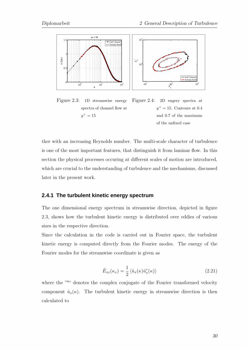
2.3 1D streamwise energy spectra of channel flow at y+ = 15 . . . . . . . . . . . 30
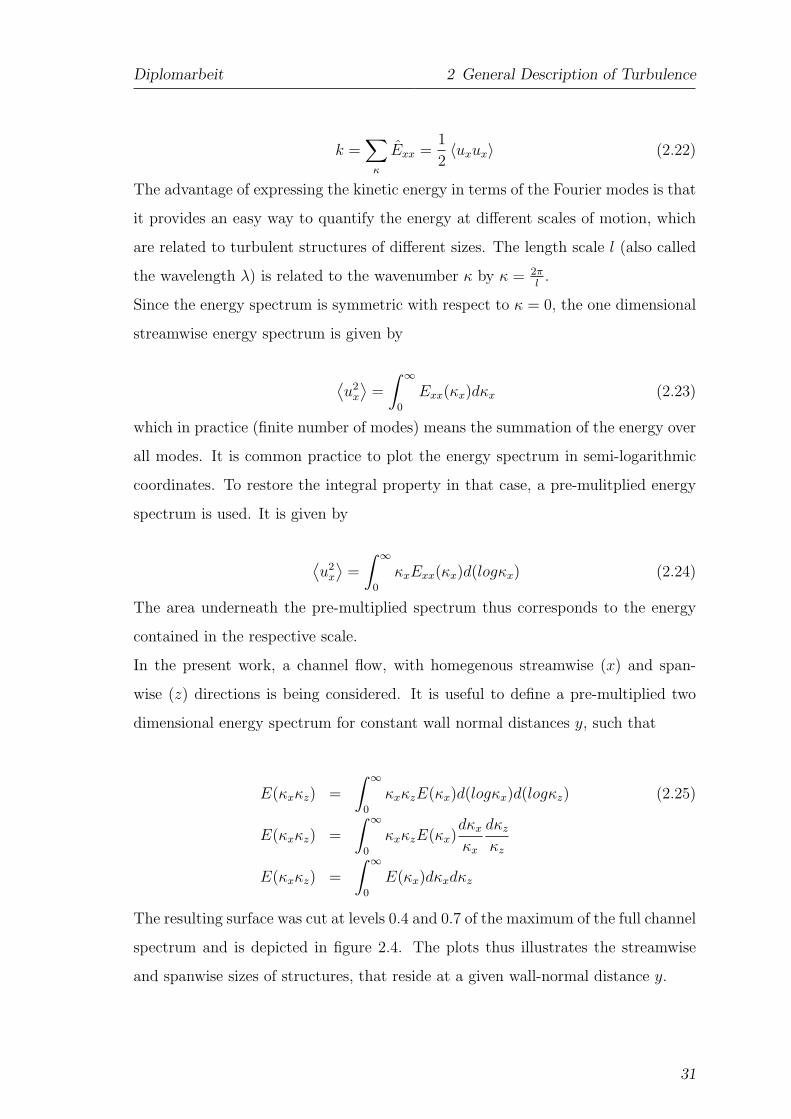
2.4 2D engery spectra at y+ = 15 . . . . . . . . . . . . . . . . . . . . . . . . 30
3.1 Channel . . . . . . . . . . . . . . . . . . . . . . . . . . . . . . . . . . 36
5.1 Computational Domain . . . . . . . . . . . . . . . . . . . . . . . . . . . 54
5.2 Channel . . . . . . . . . . . . . . . . . . . . . . . . . . . . . . . . . . 55
5.3 Mean profile and total stress for various channel sizes . . . . . . . . . . . . 57
5.4 Fit of Cess formula to “Torroja” profile . . . . . . . . . . . . . . . . . . . 60
5.5 Variation of A and κ . . . . . . . . . . . . . . . . . . . . . . . . . . . . 61
5.6 Variation of mean velocity profile . . . . . . . . . . . . . . . . . . . . . . 62
5.7 Zoomed-in view of figure on the left . . . . . . . . . . . . . . . . . . . . . 62
5.8 Mean velocity profiles . . . . . . . . . . . . . . . . . . . . . . . . . . . 62
5.9 Zoomed in view of left graph . . . . . . . . . . . . . . . . . . . . . . . . 62
5.10 Blending of two mean profiles . . . . . . . . . . . . . . . . . . . . . . . . 65
5.11 β = −0.5 blendings and their first derivative for Reτ = 550 . . . . . . . . . . 66
5.12 β = −1.0 blendings and their first derivative for Reτ = 950 . . . . . . . . . . 67
6.1 Statistics for fixed mean velocity profile at Reτ = 550 . . . . . . . . . . . . 70
6.2 Statistics for β = −0.5 and β = −1.0 profiles . . . . . . . . . . . . . . . . 71
6.3 Comparison of Reynolds stress for Reτ = 550 and Reτ = 950 cases . . . . . . 72
9
Diplomarbeit List of Figures
6.4 Isotropy coefficients and structure coefficients . . . . . . . . . . . . . . . . 73
6.5 2D streamwise velocity spectra . . . . . . . . . . . . . . . . . . . . . . . 75
6.6 2D streamwise vorticity spectra . . . . . . . . . . . . . . . . . . . . . . . 75
6.7 Pre-multiplied 1D spectra of TKE . . . . . . . . . . . . . . . . . . . . . 77
6.8 Energy in zero modes of streamwise direction . . . . . . . . . . . . . . . . 78
6.9 Energy in zero modes of wall normal direction . . . . . . . . . . . . . . . . 78
6.10 Energy in zero modes of spanwise direction . . . . . . . . . . . . . . . . . 79
6.11 Statistics of β = −0.5 blendings . . . . . . . . . . . . . . . . . . . . . . . 80
6.12 Statistics of β = −1.0 blendings . . . . . . . . . . . . . . . . . . . . . . . 81
6.13 Structure coefficient and fluctuations . . . . . . . . . . . . . . . . . . . . 81
6.14 Comparison of Reynolds stress for Reτ = 550 and Reτ = 950 cases . . . . . . 82
6.15 Energy in streamwise zero modes for blendings . . . . . . . . . . . . . . . 83
6.16 2D spectral results of the streamwise velocity . . . . . . . . . . . . . . . . 84
6.17 2D spectral results of the ωz vorticity component . . . . . . . . . . . . . . 85
6.18 Intersection of Reynolds stresses . . . . . . . . . . . . . . . . . . . . . . 87
6.19 Mean profile and mean shear of the “intersection” analysis . . . . . . . . . . 87
6.20 Total stress of the “intersection” analysis . . . . . . . . . . . . . . . . . . 88
6.21 Total stress√
τtotal for blending cases . . . . . . . . . . . . . . . . . . . . 90
6.22 Normalized streamwise velocity fluctuations . . . . . . . . . . . . . . . . . 91
6.23 Normalized wall normal velocity fluctuations . . . . . . . . . . . . . . . . . 91
6.24 Normalized spanwise velocity fluctuations . . . . . . . . . . . . . . . . . . 91
6.25 Normalized streamwise velocity fluctuations . . . . . . . . . . . . . . . . . 92
6.26 Normalized wall normal velocity fluctuations . . . . . . . . . . . . . . . . . 92
6.27 Normalized spanwise velocity fluctuations . . . . . . . . . . . . . . . . . . 92
6.28 Comparison of 950 and 550 cases . . . . . . . . . . . . . . . . . . . . . . 93
6.29 Total stresses and extra energy . . . . . . . . . . . . . . . . . . . . . . . 97
6.30 Statistics of β = −0.5 blendings . . . . . . . . . . . . . . . . . . . . . . . 98
6.31 Statistics of β = −0.5 blendings . . . . . . . . . . . . . . . . . . . . . . . 98
6.32 Spectrum of Eigenvalues for a given pertubation . . . . . . . . . . . . . . . 101
6.33 Maximum linear transient amplification of perturbations . . . . . . . . . . . 102
6.34 Comparison calculation technique of linear stability analysis . . . . . . . . . 104
10

Diplomarbeit List of Figures
6.35 Stadard Deviation of D for various cases . . . . . . . . . . . . . . . . . . 107
6.36 Visualisation of clusters . . . . . . . . . . . . . . . . . . . . . . . . . . 108
6.37 Histograms of clusters . . . . . . . . . . . . . . . . . . . . . . . . . . . 109
6.38 Joint p.d.f. of attached and detached clusters at Reτ = 550 . . . . . . . . . . 110
6.39 Joint p.d.f. of attached clusters at Reτ = 950 . . . . . . . . . . . . . . . . 112
6.40 Statistics for fixed mean velocity profile at Reτ = 550 . . . . . . . . . . . . 113
6.41 2D streamwise velocity spectra . . . . . . . . . . . . . . . . . . . . . . . 114
6.42 Energy during release of mean profile . . . . . . . . . . . . . . . . . . . . 115
11
List of Tables
5.1 Summary of box sizes . . . . . . . . . . . . . . . . . . . . . . . . . . . 54
5.2 Flow quantities of 550 channel . . . . . . . . . . . . . . . . . . . . . . . 63
5.3 Flow quantities of 950 channel . . . . . . . . . . . . . . . . . . . . . . . 64
5.4 Summary of blending cases for 550 channel . . . . . . . . . . . . . . . . . 67
5.5 Summary of blending cases for 950 channel . . . . . . . . . . . . . . . . . 68
6.1 Summary of cases for transient linear stability analysis . . . . . . . . . . . . 104
6.2 Summary of fitted parameter for transient linear stability analysis . . . . . . 104
12

Nomenclature
Arabic Symbols
1D One Dimensional
2D Two Dimensional
f Instantaneous value of forcing term
u Instantaneous velocity component in x-direction
v Instantaneous velocity component in y-direction
w Instantaneous velocity component in z-direction
A Cess parameter
a Acceleration
b Channel width
C Cascade power law constant
D Discriminant of velocity gradient
D′ Standard deviation of discriminant of velocity gradient field
dt Time differential
E Energy
13
Diplomarbeit
ETT Eddy turnover time
F Mean value of forcing term
f Fluctuation of forcing term
FFT Fast Fourier Transform
FFT Fast fourier transform
H Convection term
h Channel half hight
h+ Channel half hight in wall units
Iu Streamwise isotropy coefficient
Iw Spanwise isotropy coefficient
K Turbulent kinetic energy
k Turbulent kinetic energy
Ka Karman constant
L Channel length
l Turbulent lenght scale
l0 Lenght scale of large eddies
Lǫ Integral length scale
m Mass
N Number of grid points
n Collocation points
NG Number of grid points
Nx Number of points in x-direction
14

Diplomarbeit
Ny Number of points in y-direction
Nz Number of points in z-direction
NOP Number of arithmetic operations
P Production
p Pressure
p.d.f. Probability density function
Pi Bezier points
Q Invariant of velocity gradient
R Invariant of velocity gradient
R.H.S. Right hand side
Re Reynolds number
Reτ Reynolds number base don the friction velocity
RMS Root mean square
T Wall time
t Time
Tm Chebyshev polynomial
Tn Chebyshev polynomial
TKE Turbulent kinetic energy
U Mean of Velocity
u Velocity fluctuation in x-direction
u′ R.M.S. of streamwise velocity fluctuation
u+ streamwise velocity component in wall units
15
Diplomarbeit
u0 Velocity scale of large eddies
uη Kolomogorov velocity scale
uτ Friction velocity
Ub Bulk Velocity
Ufalse Unnatural streamwise mean velocity profile
Utrue Natural streamwise mean velocity profile
v Velocity fluctuation in y-direction
v′ R.M.S. of wall-normal velocity fluctuation
Vclus Volume of cluster
w Velocity fluctuation in w-direction
w′ R.M.S. of spanwise velocity fluctuation
x Streamwise coordinate
Y With channal half hight h normalized wall normal coordinate
y Wall normal coordinate
y+ Wall normal distance in wall units
z Spanwise coordinate
Greek Symbols
β Profile mixing variable
∆t Time increment
∆x Spatial increment
∆ Increment
16

Diplomarbeit
δv Viscious length scale
ǫ Dissipation
η Kolomogorov length scale
η+ Kolmogorov length scale in wall units
κ Wave Number and Cess parameter
κ0 Wave number of zero modes
λ Wavelength
µ Dynamic viscosity
ν Kinematic viscosity
νtot Eddy viscosity
ω Vorticity
ρ Density
τ Shear stress
τ0 Time scale of large eddies
τη Kolomogorov time scale
τw Wall shear stress
θ Chebyshev variable
17
1 Introduction
The world around us is turbulent. In nature, turbulence is the norm, not the
exception - from the smoke of a cigartte, to stormy winds, to tumultuous flood
waters, to rivers and water falls, turbulence is everywhere and has captured the
attention of many researchers in the past century. In engineering applications
turbulent flows are omnipresent and of great interest to companies whose products
are influenced by or operate in fluids in motion. The flow of the air over an aircraft
wing, blood flow in arteries, oil transport in pipelines, lava flow after a volcano
eruption, atmospheric and oceanic currents or stellar nebula as well as the mixing of
fuel and air in combustion chambers of gas turbines, we are surrounded by, and make
use of turbulence in our daily life. Understanding the nature of turbulence allows
us to influence, control it and take advantage of it by for example enhancing mixing
in processes which would not be feasible without its presnece. Thus saving money
and resources through minimizing losses due to friction, imperfect combustion and
other forms of energy dissipation. According to [6] about half the energy spent
worldwide to move fluids around or to move vehicles through fluids, is dissipated
by turbulence in the immediate vicinity of the wall.
Turbulence or turbulent flow is characterized by chaos. A set of equations, namely
the Navier- Stokes Equations, give a complete description of the turbulent flow.
Though, their strength to describe every detail of the flow becomes their burden,
since they result in fairly complex behavior and analytical solutions to even the
simplest turbulent flow problems do therefore not exist. The flow variables as a
function of space and time can only be obtained numerically. The most accurate,
though also by far the most expensive technique (resolving all time and lengths scales
18
Diplomarbeit 1 Introduction
relevant to turbulence) to simulate a flow numerically, is called Direct Numerical
Simulation, or in short DNS. It is used in the present work to compute the flow
in a channel to study the influence of a fixed mean profile on the quantities such
as velocity fluctuations and structures. This way the mechanisms of how energy is
drawn from the mean flow and fed into smaller scales is studied.
Even though DNS is the most exact tool to calculate turbulent flow, it is not
applicable for engineering computations, due to its computational cost. The en-
gineering computation relies on simpler methods such as the computationally cheap
Rynolds-averaged Navier-Stokes (RANS) simulations or Large Eddy simluations
(LES), which are intermediate in complexity between RANS and DNS. Describing
the flow variables statistically leads to the notorious closure problem, which can
only be overcome by modelling the terms, that cannot be calculated directly. The
search for improved models through a better understanding of physical phenomena
is the main objective of modern day turbulence research.
In the early days of turbulence research those models were solely based on ex-
perimental data from channel experiments. Though, with the large increase in
computational power during the last two decades, DNS has become a strong and
impressive research tool. The power of DNS not only lies within obtaining the flow
variables in a high resolved threedimensional domain, but also in the capability of
studying unphysical flow phenomena and therefore testing, validating and improving
current understandings of turbulence and its underlying mechanisms. One such
unphysical phenomena is to fix the velocity profile of the mean flow while letting
the fluctuations evolve freely. In the present work, this feature was implemented in a
fully spectral, incompressible DNS code, to evaluate its influence on flow quantities
and turbulent structures in a fully developed channel flow at Reynolds numbers
based on the friction velocity of Reτ = 550 and Reτ = 950, respectively.
The work is structured as follows. After an introductory characterization of tur-
bulence and the motivation for the present work, the mathematical equations that
19
Diplomarbeit 1 Introduction
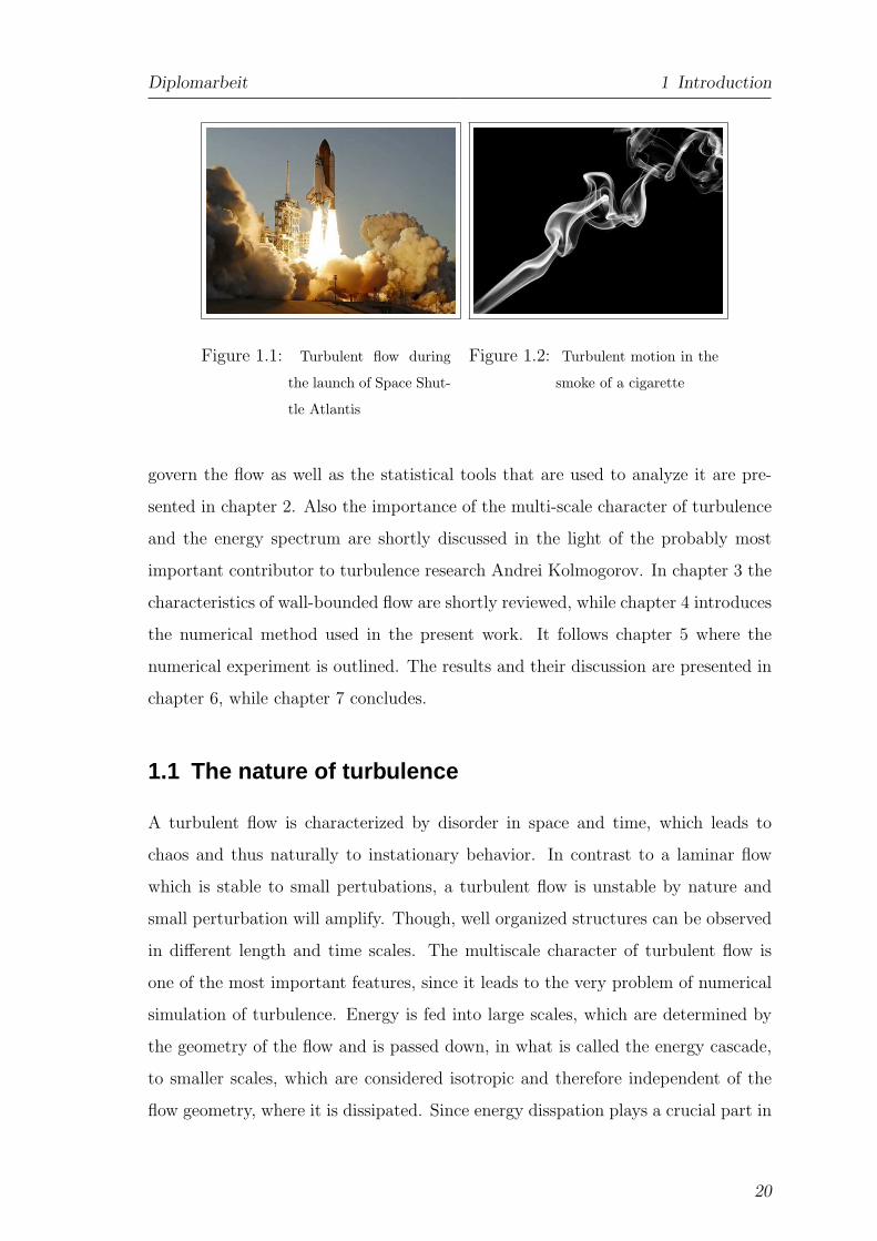
Figure 1.1: Turbulent flow during
the launch of Space Shut-
tle Atlantis
Figure 1.2: Turbulent motion in the
smoke of a cigarette
govern the flow as well as the statistical tools that are used to analyze it are pre-
sented in chapter 2. Also the importance of the multi-scale character of turbulence
and the energy spectrum are shortly discussed in the light of the probably most
important contributor to turbulence research Andrei Kolmogorov. In chapter 3 the
characteristics of wall-bounded flow are shortly reviewed, while chapter 4 introduces
the numerical method used in the present work. It follows chapter 5 where the
numerical experiment is outlined. The results and their discussion are presented in
chapter 6, while chapter 7 concludes.
1.1 The nature of turbulence
A turbulent flow is characterized by disorder in space and time, which leads to
chaos and thus naturally to instationary behavior. In contrast to a laminar flow
which is stable to small pertubations, a turbulent flow is unstable by nature and
small perturbation will amplify. Though, well organized structures can be observed
in different length and time scales. The multiscale character of turbulent flow is
one of the most important features, since it leads to the very problem of numerical
simulation of turbulence. Energy is fed into large scales, which are determined by
the geometry of the flow and is passed down, in what is called the energy cascade,
to smaller scales, which are considered isotropic and therefore independent of the
flow geometry, where it is dissipated. Since energy disspation plays a crucial part in
20
Diplomarbeit 1 Introduction
a turbulent flow, the spatial discritization has to be very fine (approach for DNS)
or a model has to be used for the small scales (approach for LES or RANS).
Turbulent flows are subject of heavy mixing, which greatly increases the transport
of matter, momentum and heat compared to laminar flow. Compared to the
turbulent diffusion, except for very close to the wall, the molecular diffusion can
be considered insignificant. From observation one will agree that turbulent flows
are rotative, which implies that vorticity (curl of velocity field) plays a major
role. Since vorticity behaves very differently in three dimensions than it does
in two dimensions, a turbulent flow has to be considered three dimensional. As
shown in [4] vorticity in two dimensions cannot be amplified, whereas for high
Reynolds number flows, in three dimensions vorticity is proportional to the angular
momentum of the fluid. Since the pressure gradient, which is the only real force in
an incompressible inviscid fluid, is irrotational and unable to influence the angular
momentum, vorticity represents a conserved quantity. Vortices are therefore good
candidates for the equivalent of objects that can be individually followed as the fluid
moves around.
Furthermore, turbulent flow is random and unpredictable, in the sense that a
small uncertainty at a given time will amplify in the manner that a deterministic
prediction of its evolution is impossible. Statistical tools as described in section 2.3
must be used to make the flow mathematically quantifiable.
Figure 1.1 shows exemplarily the nature of turbulence. The seemingly chaotic
exhaust during the launch of the Space Shuttle Atlantis exhibits turbulent motions
at different length scales. In figure 1.2 the flow of the cigarette smoke enters the
picture in a laminar motion (lower left corner) and transitions into chaotic motion:
Turbulence.
21
Diplomarbeit 1 Introduction
1.2 Motivation for current work
The motivation to fix the mean profile of the streamwise velocity component of
a turbulent channel flow originally arose from the desire to reduce the computing
time to obtain a converged solution of the turbulent flow field. Especially the
large scale structures, which for example for a channel flow are well know, take
expensive computing time to reach a converged state, while the smaller scales, due
to smaller time scales with which they are associated, reach the converged state
faster. Once the smaller structures had adapted to the larger structures, everything
could be released to compute the actual flow. Unfortunately this procedure did
not work but resulted in unexpected growth in the Reynolds stresses. It was
decided to investigate this phenomenon systematically and in greater detail, which
is the subject of the present work. A fixed mean profile, which can be interpreted
as an inverse RANS simulation since everything except for the mean profile is
calculated, was implemented in a fully spectral, incompressible DNS code, to study
the interaction between the mean flow and the fluctuations of turbulent motion.
That once the energy resides in the fluctuations, it is clear that it gradually moves
down through the energy cascade to smaller scales, where it is eventually dissipated.
However the mechanism, with which the fluctuations draw energy from the mean
profile and to what extend the Reynolds stresses and the mean velocity gradient
interact to produce turbulence is still subject of current investigation and not yet
very well understood. The hope of the present work is to find some further evidence
on how this interaction might work.
22
2 General Description of Turbulence
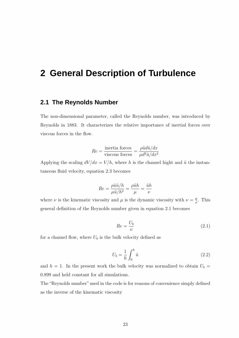
2.1 The Reynolds Number
The non-dimensional parameter, called the Reynolds number, was introduced by
Reynolds in 1883. It characterizes the relative importance of inertial forces over
viscous forces in the flow.
Re =inertia forces
viscous forces=
ρudu/dx
µd2u/dx2
Applying the scaling dV/dx = V/h, where h is the channel hight and u the instan-
taneous fluid velocity, equation 2.3 becomes
Re =ρuu/h
µu/h2=
ρuh
µ=
uh
ν
where ν is the kinematic viscosity and µ is the dynamic viscosity with ν = µρ. This
general definition of the Reynolds number given in equation 2.1 becomes
Re =Ub
ν(2.1)
for a channel flow, where Ub is the bulk velocity defined as
Ub =1
h
∫ h
0
u (2.2)
and h = 1. In the present work the bulk velocity was normalized to obtain Ub =
0.899 and held constant for all simulations.
The“Reynolds number”used in the code is for reasons of convenience simply defined
as the inverse of the kinematic viscosity
23
Diplomarbeit 2 General Description of Turbulence
Re =1
ν(2.3)
and therefore slightly higher then the acutal Reynolds number based on the bulk
velocity.
A flow is considered laminar for Re < 1, 350 and fully turbulent for Re > 1800
as stated in [1]. Since the flow for the current work reaches Reynolds numbers of
Re > 10000, the channel can be considered fully turbulent.
Several other definitions of Reynolds numbers, using different velocities, can be
defined. For the turbulent channel flow the friction velocity
uτ =
√
τw
ρ(2.4)
with the wall shear stress τw defined as
τw = ρν
(
dU
dy
)
y=0
(2.5)
where U denotes the mean velocity, is commonly used to define the friction Reynolds
number
Reτ =uτh
ν(2.6)
The friction Reynolds number of the simulations in the current work is held constant
at Reτ = 550 and Reτ = 950, respectively.
2.2 The equations of fluid motion
Applying the Navier-Stokes equations, the fluid is assumed to behave as a continous
medium. The so called continuum hypothesis holds for turbulent flow since the
smallest length and time scales encountered in turbulence are still several oders
of magnitude larger than the molecular scales. In this chapter the incompressible
(ρ = const = 1) equations of basic fluid dynamics are presented. The velocity is
24
Diplomarbeit 2 General Description of Turbulence
assumed to be sufficiently low to omit the influence of compressibility. Therefore
the continuity equation and the momentum equations completely describe the flow
field.
2.2.1 The continuity equation
The conservation of mass is given by
∂ρ
∂t+ ∇ · (ρu) = 0 (2.7)
Where u is the fluid velocity and for constant density flow this yields
∇ · u = 0 (2.8)
which means that the flow is divergence-free or solenoidal.
2.2.2 The momentum equation
The conservation of momentum is based on Newtons’ second law: F = m · a. It
relates acceleration of fluid particles to the surface and body forces experienced by
the fluid. Neglecting gravity and for now any kind of body forces (later a body
force will be added by fixing the mean profile), the only remaining force is the stress
tensor τij, which in defined, assuming a Newtonian fluid, as
τij = −pδij + µ
(
∂ui
∂xj
+∂uj
∂xj
)
(2.9)
where µ is the dynamic viscosity and p the pressure. With equation 2.8 the shear
stress τij is comprised of the sum of the isoptropic contribution −pδij and the
diviatoric contribution µ(
∂ui
∂xj+
∂uj
∂xi
)
.
According to the momentum equation, forces cause the fluid to accelerate and it
follows
25
Diplomarbeit 2 General Description of Turbulence
ρDui
Dt=
∂τij
∂xj
ρ∂ui
∂t+ ρuj
∂ui
∂xj
=∂τij
∂xj
(2.10)
or with 2.9
∂ui
∂t+ uj
∂ui
∂xj
= − ∂p
∂xi
+ ν∂2ui
∂x2i
(2.11)
where ν = µ/ρ is the kinematic viscosity. This set of equations is called the Navier-
Stokes equations and together with the continuity equation 2.8 it governs the flow
of a fluid, no matter laminar or turbulent.
2.3 Statistical description of turbulent flow
Since the turbulent velocity field of a fluid flow is random, statistical methods have
to be used to describe it. Even though the underlying Navier-Stokes equations
are a deterministic set of equations, turbulent flows display a strong sensitivity to
unavoidable perturbations in initial conditions, boundary conditions and material
properties and thus result in the random nature of turbulence. In order to quantify
turbulent flow, statistical methods are necessary. Furthermore the use of statistics
decrease the amount of data of a simulation, being considered, drastically. Imple-
menting the computation of statistics in the code reduces the size of output files
and thus make them easier and more economic to handle and to post process.
In this chapter an overview of the statistical tools and notation, used in the present
work is given.
2.3.1 Reynolds decomposition
Describing turublent velocity fields, a velocity component u is commonly split up
into a mean value U plus a fluctuation u.
u = U + u (2.12)
26
Diplomarbeit 2 General Description of Turbulence
This is called the Reynolds decomposition. Plugging the Reynolds decomposition
into the equation for mass conservation 2.8 yields
∇ · U = 0 (2.13)
and
∇ · u = 0 (2.14)
which means that both, the mean of the velocity and its fluctuation are solenoidal.
The actual problem of turbulence modelling arises from the non-linear term in the
momentum equation. The Reynolds decomposition applied to the conservation of
momentum 2.11 yields the equation for the mean flow
DUi
Dt= − ∂p
∂xj
+ ν∇2Ui −∂uiuj
∂xj
(2.15)
The only (but crucial) difference to the Navier-Stokes equations given in 2.11 are
the covariances of the velocity fluctuations 〈uiuj〉, which are called the Reynolds
stresses. The tensor 〈uiuj〉 is commonly referred to as the Reynolds stress tensor.
Without the presence of this tensor the equations of u and U would be the same.
Therefore, the different behaviour in turbulent motion is attributable to the ap-
pearance of the Rynolds stresses. Since the smallest scales of motions of turbulent
fluctuations are very small and even decrease with an increasing Reynolds number,
the requirements for the resolution are very high. Thus, the only approach that can
resolve the Reynolds stresses correctly is the direct numerical simulation (DNS).
For all other modelling techniques no closed solution of the Navier-Stokes equations
is feasable. The Reynolds stress tensor has to be modeled, which results in the
notorious “closure problem”. Since in the present work DNS is used, no further
comments on the modelling of the Reynolds stresses will be given.
2.3.2 The mean
The solution of one realisation of the flow field yields the instantaneous velocity u.
For the current situtation where the boundary conditions are independent of time
27
Diplomarbeit 2 General Description of Turbulence
the ensemble average (or mean) U of the velocity u for N independent realisations
of the flow field is calculated by
U =1
N
i∑
1
ui(x) (2.16)
where ui(x) denotes the instantaneous velocity component of the ith realisation.
The value of a mean quantity is marked by 〈·〉, except for the velocity components,
which are written in capital letters, if it is referred to the mean. In addition to
averaging over N realizations, the flow variables are averaged over homogeneous
directions (streamwise (z) and spanwise (x) directions), to improve the statistics,
since by definition flow variables are invariant under any translation in homogenous
direction. The fluctuation u is obtained by subtracting equation 2.12 from equation
2.16.
It is important to notice that the mean of a fluctuation is zero,
〈u〉 = 0 (2.17)
while the mean of a fluctuation multiplied with a fluctuation (or itself for that
matter) is not equal zero
〈uu〉 6= 0 (2.18)
This yields the famous closure problem of turbulence. Furthermore, the mean of
the mean is obviously equal to the mean
〈U〉 = U (2.19)
Those rules are used throughout the present work without further notice.
2.3.3 Statistics for the Channel Experiment
In order to obtain correct statistics a converged state of the flow has to be reached
(fully developed channel flow). A converged state was defined as a near linear profile
28
Diplomarbeit 2 General Description of Turbulence
0 0.2 0.4 0.6 0.8 10
0.5
1
τ xy+
y/h
Figure 2.1: Total Stress
0 100 200 300 400 5000.02
0.025
0.03
0.035
0.04
0.045
<vw
>
T
Figure 2.2: Diviatoric Reynolds
stress
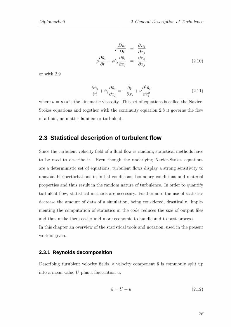
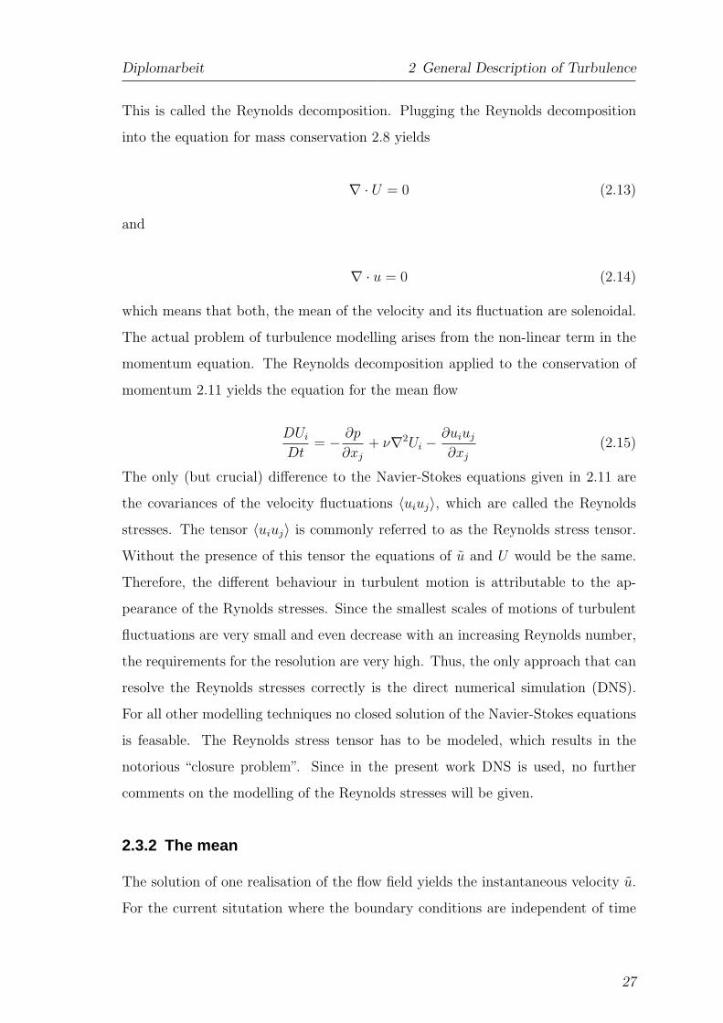
of the total stress as depicted in figure 2.1. In the present channel this takes about
5 eddy-turn-overs-times (ETT). The eddy-turn-over-time is calculated by
ETT =T · uτ
h(2.20)
where T is the wall-time of the simulation, uτ is the friction velocity and h the
channel half hight. For the current simulations this means to discard about the first
40% of the computed data to be on the safe side. Besides the linear profile of the
total stress, another good indicator whether the converged state has been reached is
the Reynolds stress 〈vw〉 which has to be constant and equal or close to zero for the
current flow configuration. Figure 2.2 depics the course of 〈vw〉 over the wall-time
T of a simulation. After fairly strong inital fluctuations 〈vw〉 settles for a value
close to zero. With uτ = 0.0488, h = 1 and ETT = 5, T is calculated to T = 100,
which if compared with figure 2.2 seems to be a fairly well converged state without
discarting an excessive amount of data.
After a steady state condition was reached, the equations were further integrated
forward in time, to obtain statistics. Statistics and spectra were calculated in the
code and written into a binary file that was then post processed using Matlab.
2.4 Scales of turbulent motion
In turbulence; a wide spectrum of length and time scales are observed, reaching in
size from the width of the flow h to very small length scales, which decrease even fur-
29
Diplomarbeit 2 General Description of Turbulence
100
101
1020
0.5
1
1.5y+ = 15
κ
κ E
(κ)
Full ChannelTorroja fixed
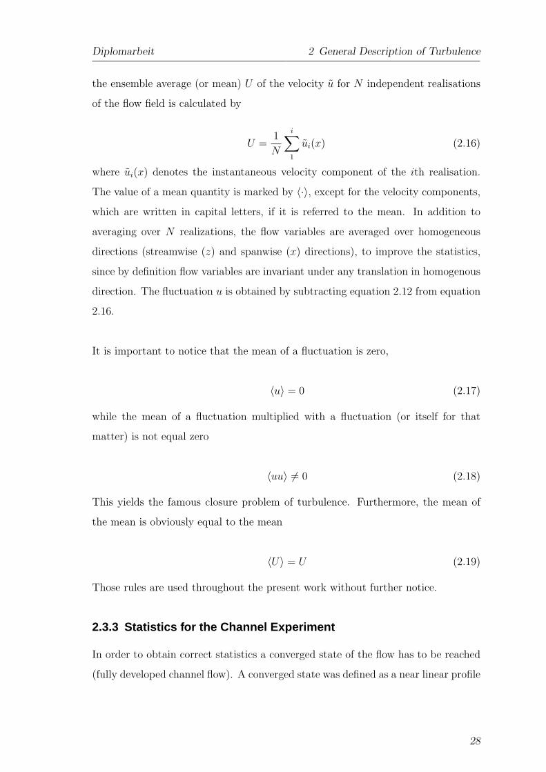
Figure 2.3: 1D streamwise energy
spectra of channel flow at
y+ = 15
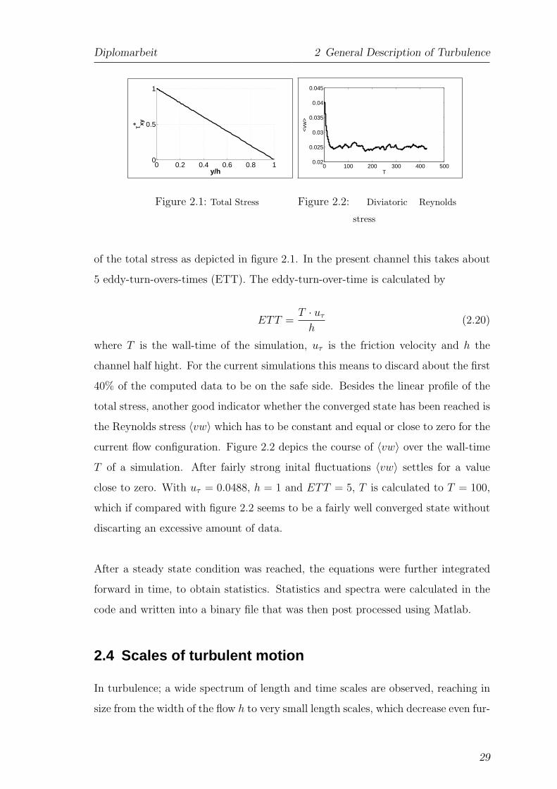
102
103
104
102
103
λ+x
λ+ z
Full ChannelTorroja fixed
Figure 2.4: 2D engery spectra at
y+ = 15. Contours at 0.4
and 0.7 of the maximum
of the unfixed case
ther with an increasing Reynolds number. The multi-scale character of turbulence
is one of the most important features, that distinguish it from laminar flow. In this
section the physical processes occuring at different scales of motion are introduced,
which are crucial to the understanding of turbulence and the mechanisms, discussed
later in the present work.
2.4.1 The turbulent kinetic energy spectrum
The one dimensional energy spectrum in streamwise direction, depicted in figure
2.3, shows how the turbulent kinetic energy is distributed over eddies of various
sizes in the respective direction.
Since the calculation in the code is carried out in Fourier space, the turbulent
kinetic energy is computed directly from the Fourier modes. The energy of the
Fourier modes for the streamwise coordinate is given as
Exx(κx) =1
2〈ux(κ)u∗
x(κ)〉 (2.21)
where the ”*“ denotes the complex conjugate of the Fourier transformed velocity
component ux(κ). The turbulent kinetic energy in streamwise direction is then
calculated to
30
Diplomarbeit 2 General Description of Turbulence
k =∑
κ
Exx =1
2〈uxux〉 (2.22)
The advantage of expressing the kinetic energy in terms of the Fourier modes is that
it provides an easy way to quantify the energy at different scales of motion, which
are related to turbulent structures of different sizes. The length scale l (also called
the wavelength λ) is related to the wavenumber κ by κ = 2πl.
Since the energy spectrum is symmetric with respect to κ = 0, the one dimensional
streamwise energy spectrum is given by
⟨
u2x
⟩
=
∫
∞
0
Exx(κx)dκx (2.23)
which in practice (finite number of modes) means the summation of the energy over
all modes. It is common practice to plot the energy spectrum in semi-logarithmic
coordinates. To restore the integral property in that case, a pre-mulitplied energy
spectrum is used. It is given by
⟨
u2x
⟩
=
∫
∞
0
κxExx(κx)d(logκx) (2.24)
The area underneath the pre-multiplied spectrum thus corresponds to the energy
contained in the respective scale.
In the present work, a channel flow, with homegenous streamwise (x) and span-
wise (z) directions is being considered. It is useful to define a pre-multiplied two
dimensional energy spectrum for constant wall normal distances y, such that
E(κxκz) =
∫
∞
0
κxκzE(κx)d(logκx)d(logκz) (2.25)
E(κxκz) =
∫
∞
0
κxκzE(κx)dκx
κx
dκz
κz
E(κxκz) =
∫
∞
0
E(κx)dκxdκz
The resulting surface was cut at levels 0.4 and 0.7 of the maximum of the full channel
spectrum and is depicted in figure 2.4. The plots thus illustrates the streamwise
and spanwise sizes of structures, that reside at a given wall-normal distance y.
31
Diplomarbeit 2 General Description of Turbulence
An approximation of the one dimensional energy spectrum in the inertial range is
given by Kolmogorov’s famous cascade power law [18]
Exx(κx) = Cǫ2/3κ−5/3 (2.26)
where C is an emperical constant. Since fairly low Reynolds numbers are used in
the present work the inertial range is not very well pronounced and this law would
only hold for a short intercept of the spectrum.
2.4.2 The energy cascade
As introduced by Richardson in 1922 the turbulent kinetic energy k is distributed
over the entire range of scales of turbulent motions. He thought of turbulence to
be composed of eddies of various sizes. Eddies are determined by the length scale
l and the time scale τ(l) = lu(l)
where u(l) is a characteristic velocity. Large eddies
can obviously contain smaller eddies with smaller time scales.
Eddies are defined as a turbulent motion within this region determined by l. The
largest eddies are of the size l0 and are determined by the geometric forcing of the
flow (e.g. channel hight h). The characteristic velocity for large eddies is in the
order of the bulk velocity Ub. The Reynolds number for the large scales is therefore
high and viscous effects are negligible.
Acording to Richardson, the kinetic energy enters the cascade at the large scales.
Those large eddies are unstable and break up, passing their energy down to some-
what smaller eddies. The smaller eddies experience the same break-up process and
energy is passed further down by inviscid processes to ever smaller scales. This is
called the energy cascade process. It is continued until the the Reynolds number
is sufficiently small (viscous forces dominate) to disspated the energy by viscous
mechanisms.
Figure 2.3 shows the pre-multiplied spectrum of the turbulent kinetic energy for the
flow analyzed in the present work. The large scales (low wave numbers) contain
most of the energy while the dissipation resides at small scales (not shown), where
the local Reynolds number is sufficiently small and therefore viscosity is active. The
size of the inertial range increases with the Reynolds number. For the Reτ = 550
32
Diplomarbeit 2 General Description of Turbulence
cases the Reynolds number is too low and the inertial range almost vanishes.
The important conclusion from the energy cascade process is, that the place for
dissipation is at the smallest scales and therefore at the end of a sequence of invicid
processes. Thus, the energy transfer is given by the first process in the sequence,
which is the energy transfer from the largest eddies to somewhat smaller eddies.
As stated above the largest eddies of the size l0 contain energy of the order u20 and
therefore a times scale τ0 = l0u0
. It follows that the rate of transfer of energy (energy
flux from larger to smaller scales) is given by
T =u2
0
τ0
=u3
0
l0(2.27)
This indicates that the rate of disspation ǫ likewise scales asu30
l0and is therefore
independent of the viscosity and subsequently indepented of the Reynolds number.
2.4.3 The Kolmogorov hypotheses
Even though Richardson answered some fundamental questions about the processes,
occuring in turbulent motion, the answer, of how small are the smallest scales and
what do they depend on, remained unanswered. The size of the smallest scales in
which dissipation takes on action is of utmost interest, since it likewise determines
the grid spacing of the numerical descritization in order to resolve those scales and
thus capture all physical phenomena of the flow. In 1941 Kolmogorov answered
those questions in what is known today as the Kolmogorov hypotheses.
The first hypothesis is called ”Kolmogorov’s hypothesis of local (small scale) isotropy“
and states that for sufficiently high Reynolds numbers, the small scales are statis-
tically isotropic. The large eddies are anisotropic and depend on the forcing of
the flow. In the break-up processes of the energy cascade the smaller eddies loose
their memory of its initial directional orientation and can therefore be considered
isotropic (invariant to arbitrary rotation and reflexion of the coordinate system).
The scales in which this hypothesis holds is called the ”universial equilibrium range“.
33
Diplomarbeit 2 General Description of Turbulence
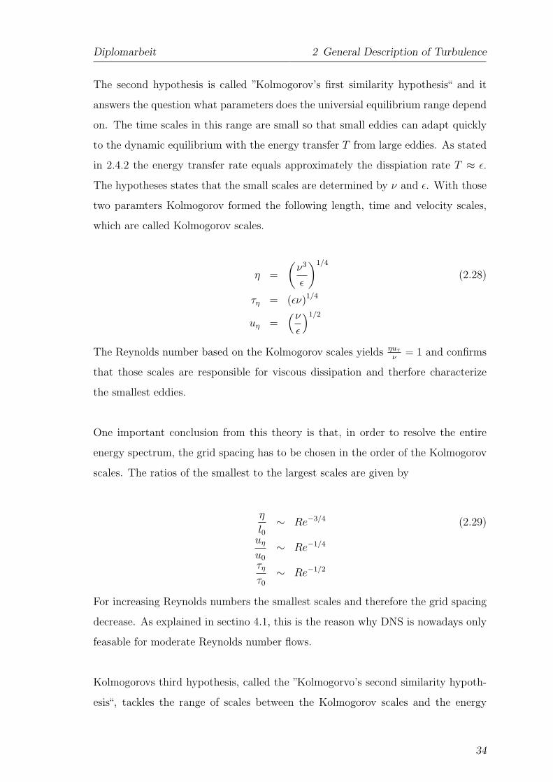
The second hypothesis is called ”Kolmogorov’s first similarity hypothesis“ and it
answers the question what parameters does the universial equilibrium range depend
on. The time scales in this range are small so that small eddies can adapt quickly
to the dynamic equilibrium with the energy transfer T from large eddies. As stated
in 2.4.2 the energy transfer rate equals approximately the disspiation rate T ≈ ǫ.
The hypotheses states that the small scales are determined by ν and ǫ. With those
two paramters Kolmogorov formed the following length, time and velocity scales,
which are called Kolmogorov scales.
η =
(
ν3
ǫ
)1/4
(2.28)
τη = (ǫν)1/4
uη =(ν
ǫ
)1/2
The Reynolds number based on the Kolmogorov scales yields ηuτ
ν= 1 and confirms
that those scales are responsible for viscous dissipation and therfore characterize
the smallest eddies.
One important conclusion from this theory is that, in order to resolve the entire
energy spectrum, the grid spacing has to be chosen in the order of the Kolmogorov
scales. The ratios of the smallest to the largest scales are given by
η
l0∼ Re−3/4 (2.29)
uη
u0
∼ Re−1/4
τη
τ0
∼ Re−1/2
For increasing Reynolds numbers the smallest scales and therefore the grid spacing
decrease. As explained in sectino 4.1, this is the reason why DNS is nowadays only
feasable for moderate Reynolds number flows.
Kolmogorovs third hypothesis, called the ”Kolmogorvo’s second similarity hypoth-
esis“, tackles the range of scales between the Kolmogorov scales and the energy
34
Diplomarbeit 2 General Description of Turbulence
containg large scales. Essentially it states that in this range (called the inertial
range) the statistics of motions are independent of the viscocity ν, since the Reynolds
number is still sufficiently high. No energy is therefore dissipated during the invicid
cascade process, but only passed down to the dissipation range.
35
3 Wall-Bounded Turbulent Flow
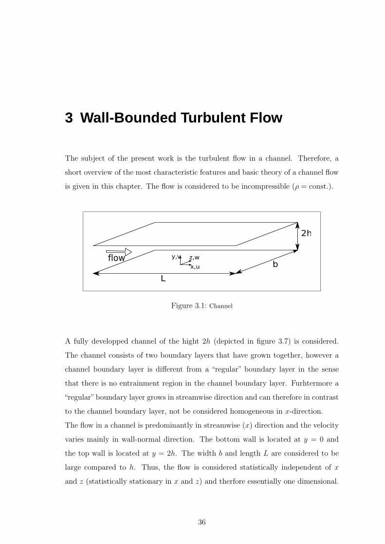
The subject of the present work is the turbulent flow in a channel. Therefore, a
short overview of the most characteristic features and basic theory of a channel flow
is given in this chapter. The flow is considered to be incompressible (ρ = const.).
L
flow
2h
bx,u
z,wy,v
Figure 3.1: Channel
A fully developped channel of the hight 2h (depicted in figure 3.7) is considered.
The channel consists of two boundary layers that have grown together, however a
channel boundary layer is different from a “regular” boundary layer in the sense
that there is no entrainment region in the channel boundary layer. Furhtermore a
“regular”boundary layer grows in streamwise direction and can therefore in contrast
to the channel boundary layer, not be considered homogeneous in x-direction.
The flow in a channel is predominantly in streamwise (x) direction and the velocity
varies mainly in wall-normal direction. The bottom wall is located at y = 0 and
the top wall is located at y = 2h. The width b and length L are considered to be
large compared to h. Thus, the flow is considered statistically independent of x
and z (statistically stationary in x and z) and therfore essentially one dimensional.
36
Diplomarbeit 3 Wall-Bounded Turbulent Flow
Furthermore the flow is symmetric about the horizontal plane y = h which is used
to furhter improve the statistics.
From the continuity equation follows with the spanwise mean velocity W = 0 that
also the wall-normal mean velocity V equals zero. Two important results from the
lateral and axial momentum equations are, that the axial pressure gradient
∂P
∂x=
dpw
dx(3.1)
is uniform along the streamwise direction and that it equals the wall-normal shear
stress gradient
dτ
∂y=
dpw
dx(3.2)
The channel flow is driven by a constant negative pressure gradient ∂P∂x
. The solution
of 3.2 results in the total shear stress with τw = τ(0)
τ(y) = τw
(
1 − y
h
)
= u2τ
(
1 − y
h
)
(3.3)
which is independet of any fluid properties. The total shear stress is the sum of the
Reynold shear stress and the viscous stress
τ(y) = −〈uv〉 + νdU
dy(3.4)
At the wall all Reynold stresses are zero and the wall shear stress only consists
of the viscous contribution. Viscosity therefore plays a crucial role near the wall,
while away from the wall the viscous stress is negligible compared to the Reynold
shear stresses. Therefore, important paramenters for the characterization of near
wall flow are the wall shear stress τw and the kinematic viscosity ν.
The friction velocity uτ is commonly used as a near wall velocity scale and is defined
as
uτ =√
τw (3.5)
and the viscous length scale is defined as
37

Diplomarbeit 3 Wall-Bounded Turbulent Flow
δv =ν
uτ
(3.6)
Quantities normalized with uτ and δv are said to be expressed in ”wall units“ and
are denoted by a ”+“ superscript. The distance from the wall measured in wall units
is
y+ =y
δv
=uτy
ν(3.7)
which can also be understood as a local Reynolds number for the size of the
structures at that hight. Low (and therfore near wall) y+ goes along with a relative
importance of viscous processes. The mean velocity expressed in wall units is given
by
U+ =U
uτ
(3.8)
3.1 Models for the near wall region
The importance of the near wall region in a turbulent channel flow becomes apparent
from the fact, that it is only near the wall where the local Reynolds number is low
enough to allow for viscous friction. The boundary layer is commonly devided into
distinct regions, which are defined by their wall-normal distance in wall units. From
the wall outwards, they are called:
The viscous sublayer (y+ < 5), the buffer layer (5 < y+ < 30), the logarithmic
(log) layer (y+ > 30) and the outer layer (y+ > 150). The first three layers are the
most characteristic features of wall-bounded turbulence [6] and constitute the main
difference between wall bounded turbulent flows and other types of turbulence.
For the detailed derivation of the models for the different regions, shortly described
in the following paragraphs, it is referred to [4] or [1]. Here only the results will be
presented.
38
Diplomarbeit 3 Wall-Bounded Turbulent Flow
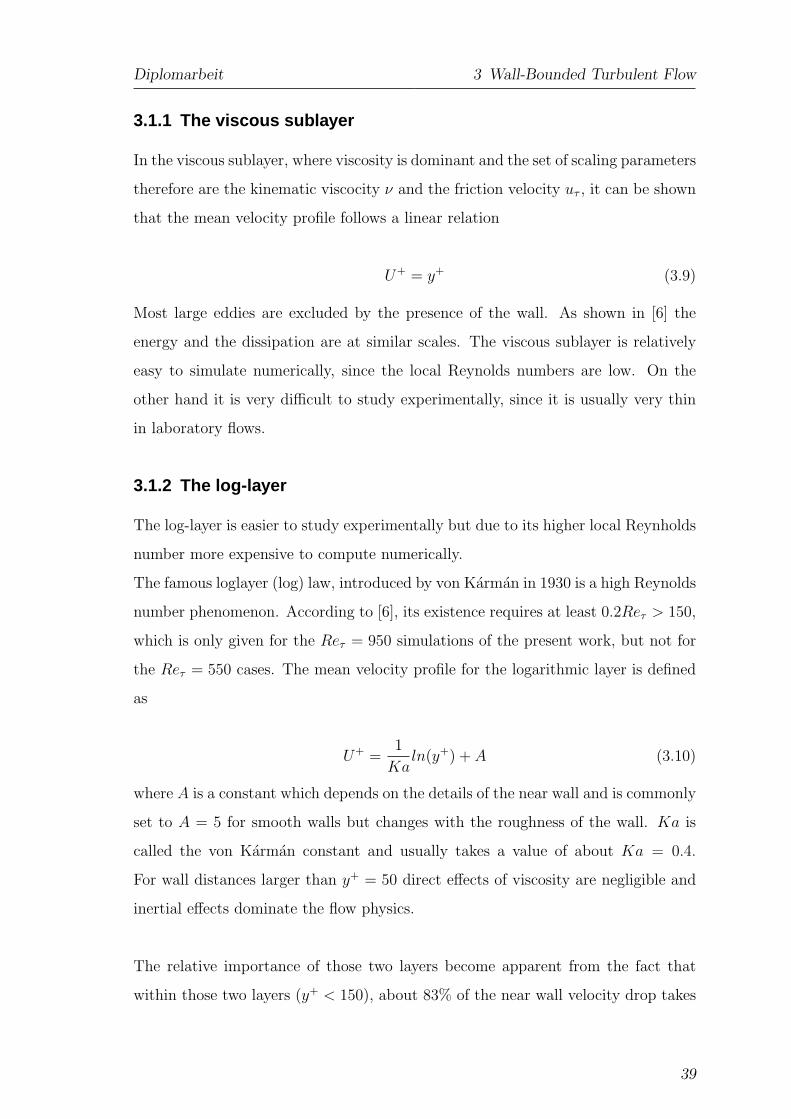
3.1.1 The viscous sublayer
In the viscous sublayer, where viscosity is dominant and the set of scaling parameters
therefore are the kinematic viscocity ν and the friction velocity uτ , it can be shown
that the mean velocity profile follows a linear relation
U+ = y+ (3.9)
Most large eddies are excluded by the presence of the wall. As shown in [6] the
energy and the dissipation are at similar scales. The viscous sublayer is relatively
easy to simulate numerically, since the local Reynolds numbers are low. On the
other hand it is very difficult to study experimentally, since it is usually very thin
in laboratory flows.
3.1.2 The log-layer
The log-layer is easier to study experimentally but due to its higher local Reynholds
number more expensive to compute numerically.
The famous loglayer (log) law, introduced by von Karman in 1930 is a high Reynolds
number phenomenon. According to [6], its existence requires at least 0.2Reτ > 150,
which is only given for the Reτ = 950 simulations of the present work, but not for
the Reτ = 550 cases. The mean velocity profile for the logarithmic layer is defined
as
U+ =1
Kaln(y+) + A (3.10)
where A is a constant which depends on the details of the near wall and is commonly
set to A = 5 for smooth walls but changes with the roughness of the wall. Ka is
called the von Karman constant and usually takes a value of about Ka = 0.4.
For wall distances larger than y+ = 50 direct effects of viscosity are negligible and
inertial effects dominate the flow physics.
The relative importance of those two layers become apparent from the fact that
within those two layers (y+ < 150), about 83% of the near wall velocity drop takes
39
Diplomarbeit 3 Wall-Bounded Turbulent Flow
place.
3.2 Dynamics of wall bounded flow
Besides the statistical description of the flow, the dynamical structures found in
turbulent flow give further insights into the mechnisms that govern turbulence.
This section focuses on the qualitative current understanding of dynamical struc-
tures found in wall bounded turbulent flow. The structures found in wall-bounded
turbulent flow are significantly different from other turbulent flows since they are
forced by the impermeability of the wall. Very long and relatively wide structures
that correlate across the whole flow thickness [10] are found in the outer layer of
turbulent wall flows. Those structures even reach into the viscous sublayer and
appear as spectral handels in the 2D spectral density plots. The box size of present
simulation, however, is too small for those structures and it is referred to simulations
of larger boxes presented for example in [11].
3.2.1 The viscous sublayer
In the near wall viscous layer the flow is relatively smooth, since because of the
low local Reynolds number, viscosity plays a major role. Eddies in this region are
within the dissipative range. Though, due to the very high mean velocity gradient
and therefore high production, the viscous layer acts like a net source of turbulent
kinetic energy (TKE), rather than a sink. The TKE production peaks customarily
in the viscous layer (around y+ ≈ 15) and is then being transported into the outer
flow regions where the production is low, due to a shallow mean velocity gradient.
As described in [4], [6] and [10], two types of structures dominate the dynamics in
the viscous layer: streamwise velocity streaks and quasi-streamwise vortices. These
structures have a well defined length scale, namely the viscosity, which allows them
to be described as individual objects. Streaks are irregular arrays of long sinuous
alternating jets, which are superimposed on the mean shear. They are about 50+
40
Diplomarbeit 3 Wall-Bounded Turbulent Flow
wide and high, and show a streamwise seperation of roughly z+ ≈ 100. Low velocity
streaks, found in the viscous sublayer (below y+ ≈ 30), are longer (up to x+ ≈ 1000)
than high velocity streaks (x+ ≈ 250), found in the buffer layer (y+ > 40). The
vortices are slightly tilded away from the wall and stay in the near wall region only
for short distances of x+ ≈ 100 before they move on into the buffer- and log-layer.
That implies, that several vortices are associated with each streak.
The dynamics near the wall are commonly thought of as a closed cycle: The vortices
cause the streaks by deforming the mean velocity gradient, thus moving high speed
fluid towards the wall and low speed fluid away from the wall. The vortices in turn
are thought to be the results of the instability of the streaks and eventual burst,
thus closing the cycle. Furthermore, from [15] it was learned, that the near wall
region is an essentially autonomous feature of the wall regions, generating turbulent
fluctuations independently of the core region. Larger structures coming from the
outer flow hardly interfere with the viscous region, since the near-wall dynamics are
strong enough to be always dominant. This indicates, that the interactions of the
streaks and the mean velocity profile by which energy is drawn from the latter one,
to feed the fluctuations, is a predominantly local process. This hypothesis will be
revisited in the course of the current proyect.
The feed-back mechanism, proposed in [12] and readily mentioned in the past
paragraph, suggests that locally weak structures, with too little Reynolds stresses,
result in a local acceleration of the mean velocity profile, which in turn leads to
local enhancement of the velocity gradient and thus to the strengthening of the local
fluctuations. Furhermore it suggests that any interaction leading to the adjustment
of the intensities of the structures at different wall distances take place between
structures of similar sizes, without necessarily passing through the mean flow. This
feedback mechanism will be challenged in the course of the current work, when the
effect of a fixed mean profile on the development of the intensities is discussed.
To furhter distinguish structures that move away or to the wall, respectively, the
so called “Quadrant” analysis is used. It devides each point of the u-v-plane into
41
Diplomarbeit 3 Wall-Bounded Turbulent Flow
quadrants. Since most of the average tangential stress is contained in the second and
forth quadrant, the resulting structures are called ejections (Q2 with u < 0, v > 0)
and sweeps (Q2 with u > 0, v < 0), respectively. Ejections cluster in groups and
are associated with individual vortices. Sweeps and ejections do not stay in the
buffer layer, but extend all the way into the log-region were, they are associated
with vortex clusters. They move fast moving fluid to the wall (sweeps) and slow
moving fluid away from the wall (ejections), thus contributing to the heavy mixing
and momentum exchange that is associated with turbulence.
3.2.2 The logarithmic region
The second region that, due to its increased local Reynolds number, only became
numerically accessible in the past decade, is the logarithmic (log) layer. For the
Reτ = 550 simulations of the present work the log-layer does not even exist, since the
upper boundary (y/h = 0.2 or y+ = 110) lies below the lower boundary (y+ = 150).
For the Reτ = 950 simulations, however, the log-layer has a small range of y+ = 40.
Simulations of higher Reynolds number such as in [11] are necessary to understand
the logarithmic region. While due to the importance of viscosity, the structures are
quite smooth near the wall, above this layer the structures have high internal local
Reynolds number of y+ >> 1 and are most likely turbulent itself. They therefore
cannot be described as single scale objects but have to be treated statistically, since
they are itself part of a turbulent cascade process. Therefore the term “eddies”
rather than vortices is used to describe them, because vorticity are usually thought
of as objects of the size of the viscous Kolmogorov length scale.
Streaks from the viscous layer have essentially disappeared above y+ = 100 and
vorticity has become isotropic, with all three components around 40η. Large struc-
tures, however, are highly anisotropic alongated mostly in streamwise direction.
Structures centered at a wall distance y are, due to their different behavior, clasified
into two categories: attached and detached eddies, depending on whether they are
42
Diplomarbeit 3 Wall-Bounded Turbulent Flow
rooted in the near wall reagion or not. Detached eddies consist of small, roughly
isotropic vortex packets that behave more or less like in free shear flow and take
part in the Kolmogorov energy cascade processes. They experience the presence of
the wall only indirectly through the shear of the mean profile.
The tall attached eddies however, are larger than y and therefore anisotropic. They
are linked to velocity structures, that are more intense than their background. Due
to the impermeability condition of the wall, which damps the wall-normal velocity
component, they do not contain tangential Reynolds stresses. As describe in greater
detail in [10] their roots must therefore be irrotational and the pressure gradient is
the only force that acts on them.
Attached eddies can be devided into “active” isotropic eddies of the size of y and
“inactive” structures of sizes much larger than y. Attached “active” isotropic eddies
are part of the classical isotropic cascade process. Every structure in the log-layer,
however, that is larger than y, is anisotropic and therefore not part of the cascade
process. Thus these inactive structures obtained their name from the fact that they
reside above the classical isotropic Kolmogorov cascade without taking part in it.
However, due to their anisotropy, they carry Reynolds stresses and also contain
most of the fluctuating turbulent energy.
In [13] a feedback mechanism, similar to the one in the near wall region, was
suggested, in which clusters are repeatedly started by wakes that were left by still
larger clusters in front of them.
43
4 The Numerical Method
Direct Numerical Simulation (DNS) was used in the present work to simulate the
turbulent flow in a channel. A short overview and some background information on
DNS, followed by the explanation of the numerical method is given in the following
chapter.
4.1 Direct Numerical Simulation
DNS has been the driving force behind the revival of turbulence research in the past
view decades [6], after numerical simulations of turbulent flows became possible in
the late 1980’s and early 1990’s due to increasing computer power. DNS provides
an unprecedented level of detail on the flow and especially for near wall regions,
where experimental measurements are difficult to carry out, it has established itself
as an indispensable research tool.
DNS solves the Navier-Stokes equations by resolving the entire spectrum of length
scales of a given flow and given boundary conditions. The resolution of the full
spectrum is needed, since, as described in chapter 2, the kinetic energy and Reynolds
stresses are associated with length scales much larger than those responsible for
energy dissipation. DNS can be seen as the numerical equivalent to experiments.
However, while experiments can be thought of as an imperfect measurement of a
true system, DNS simulations would be a perfect measurement of an approximation.
The turbulent flow field is unsteady, as in a real flow and only smooth for length
scales smaller than 10η. This means that in order to resolve those small structures
the grid of DNS has to be very fine and powerful computers are needed. The smallest
44
Diplomarbeit 4 The Numerical Method
structures decrease with increasing Reynolds number and are proportional to Re3/4.
In a three dimensional domain that yields NG ∼ Re9/4, where NG are the number
of grid points needed to resolve the smallest structures. Two orders of magnitude
have to be added to account for the time resolution and thus the total number of
arithmetic operations that need to be computed to obtain meaningful statistics are
NOP ∼ Re11/4. In other words, an increase of the Reynolds number by the factor of
10, yields an increase of the factor of 500 in the number of arithmetic operations.
Even though the underlying Navier-Stokes equations have been known for over a
century, because of the requirements stated above, DNSs of turbulent flows were
unfeasible until the late 1980s when computers with sufficient capabilities became
available.
Conceptually DNS is the simplest approach, since no model is used and the entire
flow field is resolved. In that sense DNS simulations have several advantages
over experiments. Once a flow has been simulated all the data is available in a
three-dimensional domain and thus post-processing allows even to compute views
and terms which are difficult to obtain by experiments. Furthermore, imaginary
”unphysical“ flow phenomena can be simulated, by mposing boundary conditions,
that differ from the natural ones, to check for processes and validate hypothesis,
that could not be obtained from experiments. This makes DNS an excellent research
tool which will expand its influence with growing hardware capabilities.
As discussed in section 2.4, the smallest structures in the turbulent flow field and
therefore the grid spacing, decrease with increasing Reynolds number. That means,
that due to a lack of sufficient computing power, only moderate Reynold numbers
can be simulated. Though, as long as the physics (separation of energy containing
scales and dissipation scales) of the flow can be represented accurately, valuable
data and insights can be obtained from the simulations available today. It must be
stressed, that the objective of DNS is not to reproduce real life flows, but rather to
use it as an academic research tool, allowing the study of flow physics and thus the
45
Diplomarbeit 4 The Numerical Method
development of improved turbulence models, which then can be used in commercial
flow solvers.
4.2 The numerical procedure
4.2.1 Derivation of the governing equations
In order to implement the equations of fluid motions, as given in 2.2, in the code
they have to be modified slightly. By doing so, continuity is imposed implicitely
and does not have to be accounted for seperately. The equations of conservation
of momentum and mass are taken from sections 2.2.2 and 2.2.1, respectively. For
reasons of simplicity and clarity the notation is chosen such that ∂x denotes the
operator ∂∂x
, etc. The convection term is denoted by Hj = ui∂uj
∂xi. Following [2], the
governing equations for the fluid can be written as
∂tuj = ∂xjp − Hj +
1
Re∇2uj (4.1)
and
∇ · u = 0 (4.2)
In order to eliminate the pressure gradient, the curl of the momentum equation 4.1
is taken and it follows
∂t (∇× uj) = ∇× Hj +1
Re∇2 (∇× uj) (4.3)
or written out for all three spatial directions
∂t [∂yuw − ∂zv] = (∂yH3 − ∂zH2) +1
Re∇2 (∂yw − ∂zv) (4.4)
∂t [∂zuu − ∂xw] = (∂zH1 − ∂xH3) +1
Re∇2 (∂zu − ∂xw) (4.5)
∂t [∂xuv − ∂yu] = (∂xH2 − ∂yH1) +1
Re∇2 (∂xv − ∂yu) (4.6)
where equation 4.5 is the equation for the normal component of vorticity ω
46
Diplomarbeit 4 The Numerical Method
∂tω = (∂zH1 − ∂xH3) +1
Re∇2ω (4.7)
Equation 4.4 is multiplied by the operator ∂z and equation 4.6 is multiplied by the
operator ∂x and subsequently equation 4.6 is subtracted from equation 4.4. This
yields
∂t
[
∂2xv + ∂2
z v − ∂x∂yu − ∂z∂yw]
= R.H.S. (4.8)
where the R.H.S. (right hand side) is given by
R.H.S. =(
∂2xH2 + ∂2
zH2 − ∂x∂yH1 − ∂z∂yH3
)
+1
Re∇2
[
∂2xv + ∂2
z v − ∂x∂yu − ∂z∂yw]
(4.9)
The conservation of mass
∇ · u = ∂xu + ∂yv + ∂zw = 0 (4.10)
is used to eliminate the terms −∂x∂yu − ∂z∂yw in equations 4.8 and 4.9 and is
therefore implicitly imposed. With equation 4.10 it follows
∂yv = −∂xu − ∂zw
∂2y v = −∂x∂yu − ∂zw (4.11)
and thus equations 4.8 and 4.9 can be written as
∂t
[
∂2xv + ∂2
z v + ∂2y v
]
= −∂y [∂xH1 + ∂zH3]+H2
[
∂2x + ∂2
z
]
+1
Re∇2
[
∂2xv + ∂2
z v + ∂2y v
]
(4.12)
or
∂t∇v = −∂y [∂xH1 + ∂zH3] + H2
[
∂2x + ∂2
z
]
+1
Re∇4v (4.13)
The code solves for the Laplacian of the wall-normal velocity component and the
normal component of the vorticity using equation 4.13 and 4.7, respectively.
47
Diplomarbeit 4 The Numerical Method
The definition of the vorticity ω = ∂zu − ∂xw and the continuity equation, given
in 4.10, are used to compute the stream- and spanwise velocity components. For
the computation, carried out using a spectral method (Fourier series in x and z
and Chebyshev ploynomial in y), all the derivatives become multiplications which
results in a favorable algebraic equation.
The price, paid for the elimination of the pressure and implicitly incorporating
the continuity equation into the Navier-Stokes equations, is the resulting 4th order
differential equation, which requires more grid points (higher computational cost)
to yield the same accuracy as a 2nd order equation. By substitution, the 4th order
equation is therefore split up into two second-order equations, to solve them more
efficiently.
For the convective terms a third order Runge-Kutta scheme is used to advance in
time. The Backward Euler Method (implicit) is used for the time advancement
of the viscous part. The Chebyshev-tau method is used to solve the discretized
equations as explained in further detail in [2].
For a constant density flow there is no connection between the pressure and the
density of the fluid and the pressure gradient is uniquely determined by the current
velocity field, independent of the flow’s history. Thus, the procedure stated above
does not require the calculation of the pressure. It was only calculated during
post processing, to obtain turbulence statistics, such as for example the budget of
the Reynolds stress, which involves pressure. It was computed from the normal
momentum equation with the wall pressure determined from the combination of
streamwise and spanwise momentum equations.
4.2.2 Initial and Boundary Conditions
Since the channel is assumed to be periodic in streamwise direction, the initial
conditions do not play a crucial role and were taken from previous analysis of
the same channel. As long as the initial condition roughly represent the large
48
Diplomarbeit 4 The Numerical Method
scale fluctuations and mean velocity profile, the channel will adapt itself. The
intermittency in stream- and spanwise direction also omits the problem of finding
adequate inflow and outflow conditions and boundary conditions, respectively. The
outflow on one side is simply recycled as the inflow on the other side, thus creating
an infinite channel length and width, respectively. Although the box size has to be
chosen sufficently large in order to represent correctly the large scale structures in
the flow.
no-slip boundary condition were implemented in wall-normal directions (equation
4.13) at y = ±1, such that
v(±1) =∂v
∂y(±1) = 0 (4.14)
4.2.3 Spectral Method
In computational fluid dynamics, finite difference or spectral methods are used
to discretize the equations of fluid motions and calculate a numerical solution of
them. Finite difference methods approximate the solution locally and thus result
in sparsly filled matrices, which can be solved using specialized methods, exploiting
the diagonal predominance. Spectral methods, instead, approximate the solution
globally with a series sum of orthogonal basis functions. A computation domain
can be dicretized using different methods in different spatial directions. For a given
number of degrees of freedom (grid points) it can be said that generally spectral
methods yield more accurate results than finite difference methods. Spectral meth-
ods perform well with fairly smooth and regular geometries but cause problems (loss
of accuracy and efficiency) in more complicated features, as commonly encountered
in industrial flows. Also, due to the necessary transformation into Fourier space,
spectral methods are more costly than finite difference methods.
The code used in the present work, uses a spectral method in all three spatial
directions. Therefore this chapter will be limited to spectral methods, which will
be presented shortly.
49
Diplomarbeit 4 The Numerical Method
Spectral methods are extremely accurate and non-dissipative tools for calculating
derivatives of descrete data sets, which is the main objective of a numerical method
when finding the solution to a differential equation. Using the complex representa-
tion given in equation 4.15, it can easily be seen that the derivative of an exponential
turns into a multiplication with its exponent. Furthermore, spectral methods enjoy
exponential convergence and thus makes it possible, if drafted correctly, to find a
highly accurate solution of a differential equation.
A spectral method approximates a function in physical space as a series sum of
orthogonal basis functions. The most common choice for an orthogonal basis
function are the Fourier series. They are used in homogeneous directions, since
the flow is assumed to be periodic in those directions, and as stated in [3] Fourier
series work best for periodic problems. The complex representation of the velocity
component u in Fourier space is given by
u(x, t) = u(κ0, t) + 2N
∑
κ=1
u(κ, t)eiκx (4.15)
with the coefficient
u(κ, t) =1
2π
∫ κmax
κ0
u(x, t)e−inxdx (4.16)
which represents component of the velocity u(x, t) in Fourier space. In the channel
experiment considered in the present work, the zero mode u(κ0, t) represents the
mean velocity profile. The fluctuation from the mean is given the second part of the
sum in equation 4.15. Furthermore, the wavenumbers are assumed to be symmetric
with respect to zero and thus only positive wavenumbers (κ = 1 to N) are considered
and multiplied by the factor 2. The largest wave number that is represented and
thus associated with the mean profile, is
κ0 =Nπ
L(4.17)
where L denotes the box size in the direction considered and N the number of
50
Diplomarbeit 4 The Numerical Method
grid points (modes) with which the respective direction was discretized. The grid
spacing in physical space is given by
∆x =L
N(4.18)
For the non-periodic wall-normal direction (y) a Chebyshev polynomal expansion is
used in the code. A Chebyshev polynomal expansion is merely a Fourier cosine series
with a change of the variable. The Chebyshev polynomial series approximation of
the wall normal velocity component is given by
v(y, t) =N
∑
n=1
v(y, t)Tm(y) − 1
2v(0, t) (4.19)
The coefficient v is defined as
v(y, t) =2
N
N∑
i=1
v(yi)Tm(yi) (4.20)
where the Chebyshev polynomial Tm of degree m, defined over the interval [−1, 1]
is given as
Tm = cos (m · arccos(y)) (4.21)
and the zeros (collocation points) of the polynomial are located at
yi = cos
(
π(i − 12)
m
)
(4.22)
for i = 1...N .
In order to keep computing costs down, a fast fourier transform (FFT) algorithm is
used for the one-to-one mapping between the Fourier coefficients and the velocities
in physical space. Further cost can be avoided by using a pseudo-spectral method.
This avoids the costly computation of the non-linear terms of the Navier-Stokes
equations by transfering the velocity field back into physical space, computing the
non-linear terms and transfering the result back into Fourier space.
51

Diplomarbeit 4 The Numerical Method
4.2.4 Spacial Resolution
The spatial resolution required, to resolve the smallest energy dissipating scales, is
determined by the flow physics (e.g. Reynolds number). The accuracy, with which
theses scales are represented is determined by the numerical method, while the grid
determines the scales that can actually be represented.
While the Kolmogorov length scale η = (ν3/ǫ)1/4 is commonly used as the smallest
scale that must be resolved, the relevant scales to obtain reliable statistics are
typically larger than that. As stated in [4] most of the dissipation occurs at scales
larger than 15η and therefore a rule of thumb states, the smallest scales must only
be in the order of the Kolmogrov scale and not necessarily equal to η.
The approximation for the Kolomogorov length scale
η = Lǫ/Re3/4 (4.23)
for the Reτ = 550 (Re = 11180) case, with Lǫ = h = 1, yields η = 0.0009, which
correspsonds to η+ = 0.495. As can be seen in table 5.1, the grid spacing in all three
spatial directions is therefore within the order of magnitude of the Kolmogorov
length scale. This makes it possible to accurately represent the physics at small
scales (vortices) which are crucial for the study turbulence.
4.2.5 Time Resolution
In turbulence not only the length scales are spread over a wide range of scales,
but also the time scales are required to be sufficiently small to account for the
smallest structures to be resolved in time. The requirement of time accuracy over
a wide range of scales does not permit large steps, as e.g. used in aerodynamic
flows, where implicit schemes allow for it. Large time steps in turbulent flow would
lead to large errors in the small scales. The range of frequencies that need to be
accurately represented are dictated by physics, while the numerical scheme used,
determines the frequencies resolved. Implicit time advancement is unconditionally
stable but also uses more resources than explicit time advancement. It therefore is
most attractive when the frequencies of the flow are far lower than those represented
52
Diplomarbeit 4 The Numerical Method
by the discrete equations. On the other hand, to achieve numerical stability with
explicit time advancement, the time step needs to be smaller than it takes for a
fluid particle to cross one grid element, which leads to the restriction that the CFL
(Courant Friedrich Levi) number cannot exceed the value of 1. The CFL number
is defined as
CFL =dtu
dx≤ 1 (4.24)
In the present simulation a CFL number of 1 is used, accounting for stability but at
the same time obtaining an economic scheme. Since, due to physics of turbulence,
time steps are required to be small anyway, the most economical solution is to use
explicit time advancement. In the present DNS code a Crank-Nicholson-Scheme
(implicit) is used for the viscous term and a Adams-Bashforth-Scheme (explicit) for
the non-linear term. In order to acquire a stable time integration, the time step has
to be determined by choosing the smaller of the viscous or the convective time step
but since the viscous term is treated implicitely (unconditionally stable), the time
step is determined by the convective part and therefore the CFL number.
4.2.6 Error
Even though as stated earlier, the spectral method used in the code, have excellent
error properties, there is one sources of error, that ought to be pointed out briefly in
this section. For spectral methods the so called ”Aliasing“ appears when computing
the nonlinear terms pseudo spectrally. It causes different modes to become indistin-
guishable and the solution therefore contains modes that are actually not present
in the flow. The anti-aliasing technique used, expands the number of collocation
points by a factor of 3/2 before transforming them into physical space.
53
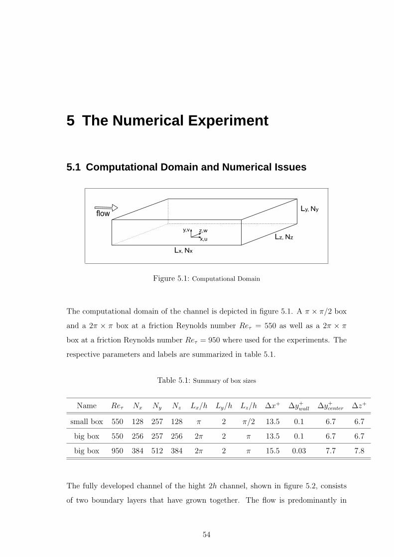
5 The Numerical Experiment
5.1 Computational Domain and Numerical Issues
Lx, Nx
flowLy, Ny
Lz, Nzx,u
z,wy,v
Figure 5.1: Computational Domain
The computational domain of the channel is depicted in figure 5.1. A π × π/2 box
and a 2π × π box at a friction Reynolds number Reτ = 550 as well as a 2π × π
box at a friction Reynolds number Reτ = 950 where used for the experiments. The
respective parameters and labels are summarized in table 5.1.
Table 5.1: Summary of box sizes
Name Reτ Nx Ny Nz Lx/h Ly/h Lz/h ∆x+ ∆y+wall ∆y+
center ∆z+
small box 550 128 257 128 π 2 π/2 13.5 0.1 6.7 6.7
big box 550 256 257 256 2π 2 π 13.5 0.1 6.7 6.7
big box 950 384 512 384 2π 2 π 15.5 0.03 7.7 7.8
The fully developed channel of the hight 2h channel, shown in figure 5.2, consists
of two boundary layers that have grown together. The flow is predominantly in
54
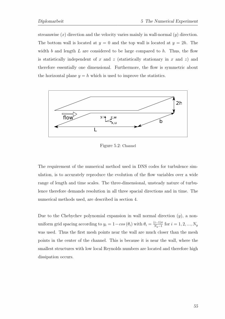
Diplomarbeit 5 The Numerical Experiment
streamwise (x) direction and the velocity varies mainly in wall-normal (y) direction.
The bottom wall is located at y = 0 and the top wall is located at y = 2h. The
width b and length L are considered to be large compared to h. Thus, the flow
is statistically independent of x and z (statistically stationary in x and z) and
therefore essentially one dimensional. Furthermore, the flow is symmetric about
the horizontal plane y = h which is used to improve the statistics.
L
flow
2h
bx,u
z,wy,v
Figure 5.2: Channel
The requirement of the numerical method used in DNS codes for turbulence sim-
ulation, is to accurately reproduce the evolution of the flow variables over a wide
range of length and time scales. The three-dimensional, unsteady nature of turbu-
lence therefore demands resolution in all three spacial directions and in time. The
numerical methods used, are described in section 4.
Due to the Chebychev polynomial expansion in wall normal direction (y), a non-
uniform grid spacing according to yi = 1−cos (θi) with θi = (i−1)πNy−1
for i = 1, 2, ..., Ny
was used. Thus the first mesh points near the wall are much closer than the mesh
points in the center of the channel. This is because it is near the wall, where the
smallest structures with low local Reynolds numbers are located and therefore high
dissipation occurs.
55
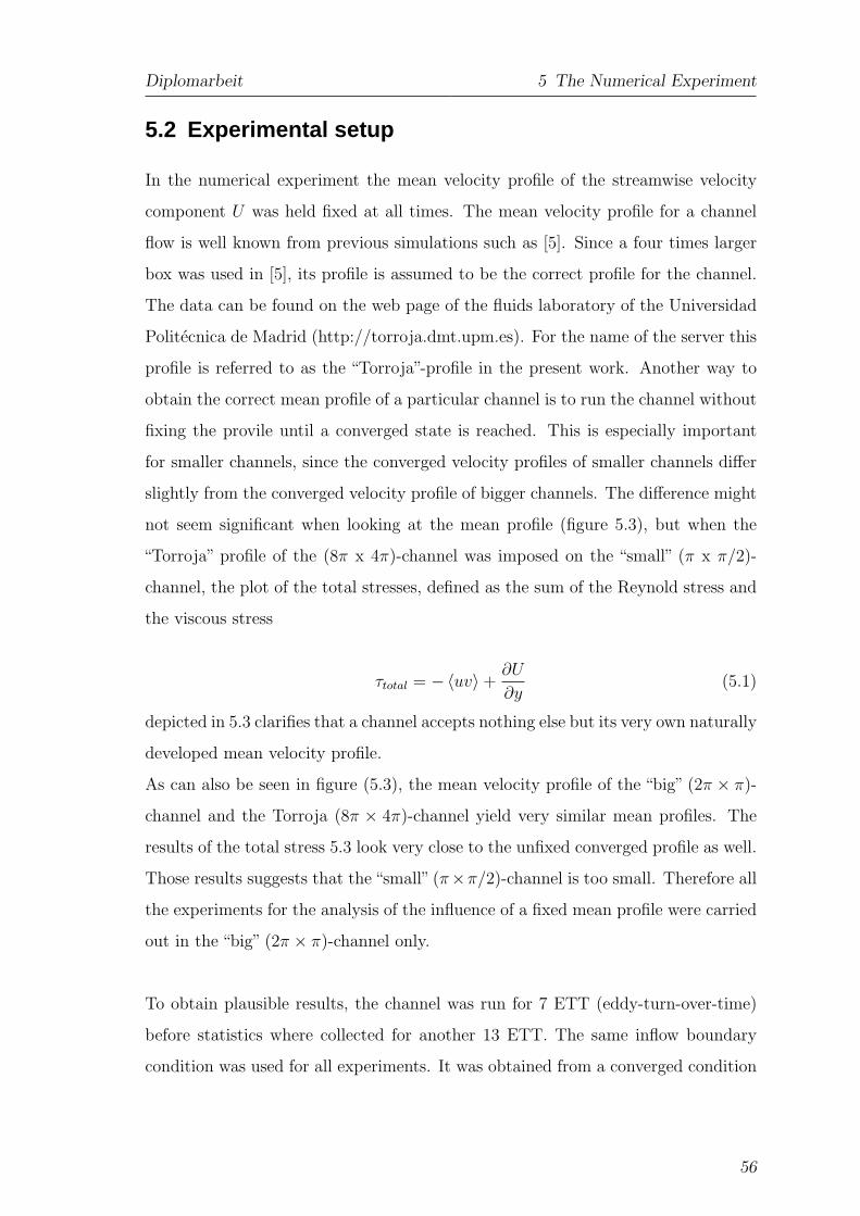
Diplomarbeit 5 The Numerical Experiment
5.2 Experimental setup
In the numerical experiment the mean velocity profile of the streamwise velocity
component U was held fixed at all times. The mean velocity profile for a channel
flow is well known from previous simulations such as [5]. Since a four times larger
box was used in [5], its profile is assumed to be the correct profile for the channel.
The data can be found on the web page of the fluids laboratory of the Universidad
Politecnica de Madrid (http://torroja.dmt.upm.es). For the name of the server this
profile is referred to as the “Torroja”-profile in the present work. Another way to
obtain the correct mean profile of a particular channel is to run the channel without
fixing the provile until a converged state is reached. This is especially important
for smaller channels, since the converged velocity profiles of smaller channels differ
slightly from the converged velocity profile of bigger channels. The difference might
not seem significant when looking at the mean profile (figure 5.3), but when the
“Torroja” profile of the (8π x 4π)-channel was imposed on the “small” (π x π/2)-
channel, the plot of the total stresses, defined as the sum of the Reynold stress and
the viscous stress
τtotal = −〈uv〉 +∂U
∂y(5.1)
depicted in 5.3 clarifies that a channel accepts nothing else but its very own naturally
developed mean velocity profile.
As can also be seen in figure (5.3), the mean velocity profile of the “big” (2π × π)-
channel and the Torroja (8π × 4π)-channel yield very similar mean profiles. The
results of the total stress 5.3 look very close to the unfixed converged profile as well.
Those results suggests that the “small” (π×π/2)-channel is too small. Therefore all
the experiments for the analysis of the influence of a fixed mean profile were carried
out in the “big” (2π × π)-channel only.
To obtain plausible results, the channel was run for 7 ETT (eddy-turn-over-time)
before statistics where collected for another 13 ETT. The same inflow boundary
condition was used for all experiments. It was obtained from a converged condition
56
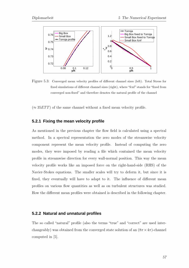
Diplomarbeit 5 The Numerical Experiment
0.08 0.1 0.12
0.72
0.73
0.74
0.75
0.76
U
y/h
Big BoxSmall BoxTorroja profile
0 0.5 10
0.2
0.4
0.6
0.8
1
1.2
τ xy+
y/h
TorrojaBig Box fixed to TorrojaSmall Box fixed to TorrojaSmall Box fcnf
Figure 5.3: Converged mean velocity profiles of different channel sizes (left). Total Stress for
fixed simulations of different channel sizes (right), where “fcnf” stands for “fixed from
converged non-fixed” and therefore denotes the natural profile of the channel
(≈ 35ETT ) of the same channel without a fixed mean velocity profile.
5.2.1 Fixing the mean velocity profile
As mentioned in the previous chapter the flow field is calculated using a spectral
method. In a spectral representation the zero modes of the streamwise velocity
component represent the mean velocity profile. Instead of computing the zero
modes, they were imposed by reading a file which contained the mean velocity
profile in streamwise direction for every wall-normal position. This way the mean
velocity profile works like an imposed force on the right-hand-side (RHS) of the
Navier-Stokes equations. The smaller scales will try to deform it, but since it is
fixed, they eventually will have to adapt to it. The influence of different mean
profiles on various flow quantities as well as on turbulent structures was studied.
How the different mean profiles were obtained is described in the following chapter.
5.2.2 Natural and unnatural profiles
The so called “natural” profile (also the terms “true” and “correct” are used inter-
changeably) was obtained from the converged state solution of an (8π×4π)-channel
computed in [5].
57
Diplomarbeit 5 The Numerical Experiment
In order to examine the influence of an unnatural mean velocity profile, the Cess
Formula [?] was used. The Cess Formula which gives an approximation of the total
(molecular plus turbulent) viscosity is defined as
νtot
ν=
1
2
[
1 +κ2h+2
9
[
2Y − Y 2]2 [
3 − 4Y + 2Y 2]2
[
1 − e−Y h+
A
]2]1/2
+1
2(5.2)
where Y is defined as Y = y/h. The mean velocity profile is then obtained by
integrating the momentum equation
∂U
∂y=
u2τ (1 − Y )
νtot
(5.3)
which can be expressed in wall units
U =
∫ y
0
u2τ (1 − Y )
νtot/ν
dy
ν
U+ =
∫ 1
0
uτ (1 − Y )
νtot/νdY
uτh
ν
U+ = Reτ
∫ 1
0
uτ (1 − Y )
νtot/νdY (5.4)
dU+
dY= Reτ
uτ (1 − Y )
νtot/ν(5.5)
With the definition of y+
y+ =yuτ
ν(5.6)
this yields
Y =y+ν
uτh
Y =y+
Reτ
dY = dy+
Reτ
(5.7)
By applying 5.7 on 5.4 it follows
58
Diplomarbeit 5 The Numerical Experiment
dU+
dY=
dU+
d y+
Reτ
=dU+
dy+Reτ = Reτ
1 − Y
νtot/ν(5.8)
and therefore
dU+
dy+=
1 − Y
νtot/ν(5.9)
Integrating 5.9 yields the mean velocity profile in wall units
U+ = Reτ
∫ 1
0
1 − Y
νtot/νdY (5.10)
where νtot/ν is obtained from the Cess formula 5.2. Equation 5.10 was integrated
numerically. For h+ = 550 and h+ = 950, respectively, the two parameters κ and
A in 5.2 were fitted to the “Torroja” profile by a least square fit. The procedure
will be explained examplarily for the Reτ = 550 case. The “Torroja” profile was
approximated well by κ = 0.46 and A = 29.90 as depicted in figure 5.4. The
collocation points for the numerical integration are given by
y = 1 − cos
(
kπ
N − 1
)
(5.11)
with k = 1...N = 257 and
Y =y
h(5.12)
The mass flux Ub, the friction Reynolds number Reτ and the nominal energy
production P/u3τ were held constant. P is defined as
P =
∫ h
0
[
u2τ (1 − Y ) − ν
∂U
∂y
]
∂U
∂ydy (5.13)
where again Y = yh. With
∂U+
∂Y= Reτ
(
1 − Y
νt/ν
)
(5.14)
it follows
59
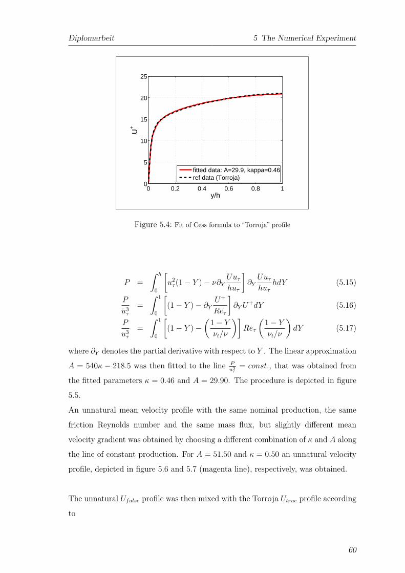
Diplomarbeit 5 The Numerical Experiment
0 0.2 0.4 0.6 0.8 10
5
10
15
20
25
y/h
U+
fitted data: A=29.9, kappa=0.46ref data (Torroja)
Figure 5.4: Fit of Cess formula to “Torroja” profile
P =
∫ h
0
[
u2τ (1 − Y ) − ν∂Y
Uuτ
huτ
]
∂YUuτ
huτ
hdY (5.15)
P
u3τ
=
∫ 1
0
[
(1 − Y ) − ∂YU+
Reτ
]
∂Y U+dY (5.16)
P
u3τ
=
∫ 1
0
[
(1 − Y ) −(
1 − Y
νt/ν
)]
Reτ
(
1 − Y
νt/ν
)
dY (5.17)
where ∂Y denotes the partial derivative with respect to Y . The linear approximation
A = 540κ − 218.5 was then fitted to the line Pu3
τ= const., that was obtained from
the fitted parameters κ = 0.46 and A = 29.90. The procedure is depicted in figure
5.5.
An unnatural mean velocity profile with the same nominal production, the same
friction Reynolds number and the same mass flux, but slightly different mean
velocity gradient was obtained by choosing a different combination of κ and A along
the line of constant production. For A = 51.50 and κ = 0.50 an unnatural velocity
profile, depicted in figure 5.6 and 5.7 (magenta line), respectively, was obtained.
The unnatural Ufalse profile was then mixed with the Torroja Utrue profile according
to
60
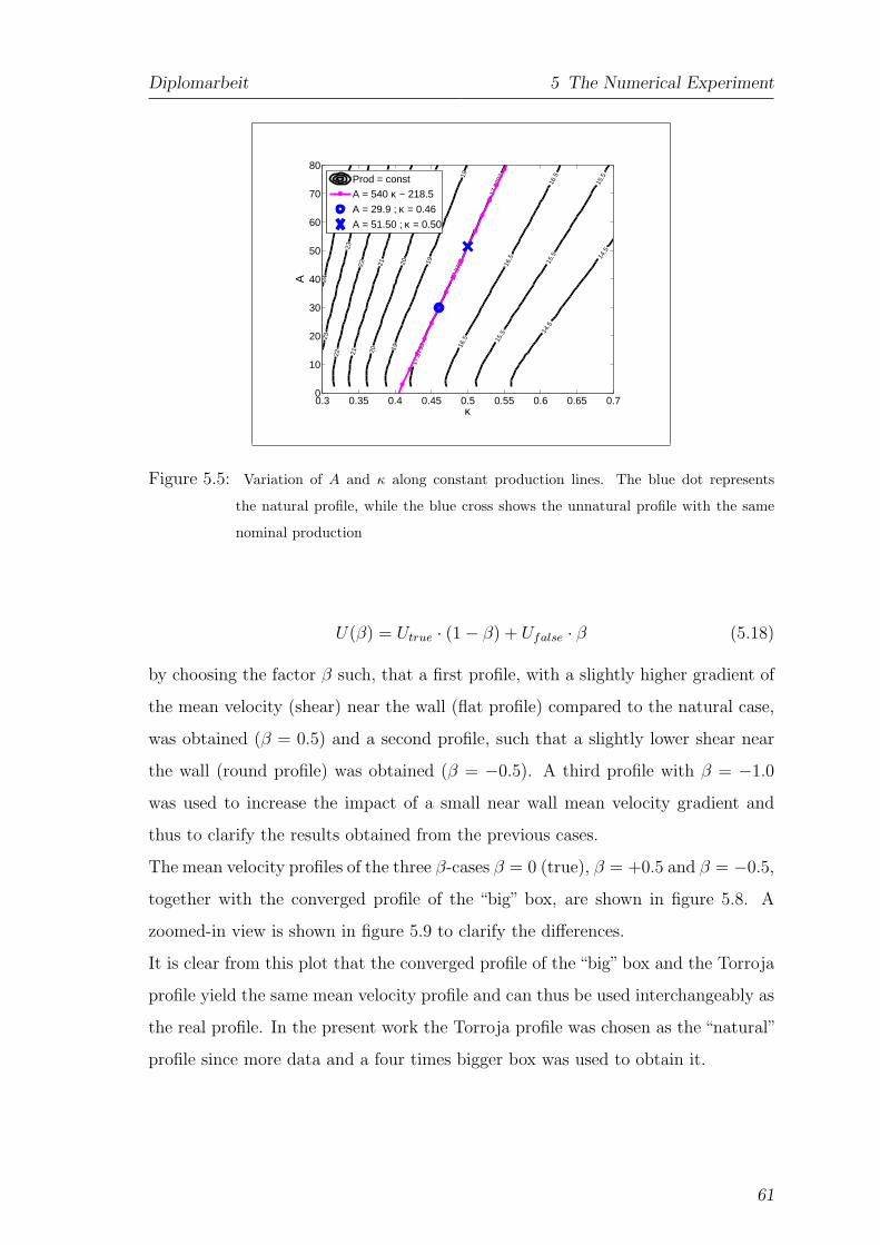
Diplomarbeit 5 The Numerical Experiment
14.5
14.5
15.5
15.5
15.5
16.5
16.5
16.5
17.8
793
17.8
793
17.8
793
19
19
19
20
20
20
21
21
21
22
22
22
23
23
24
24
κ
A
0.3 0.35 0.4 0.45 0.5 0.55 0.6 0.65 0.70
10
20
30
40
50
60
70
80Prod = const
A = 540 κ − 218.5
A = 29.9 ; κ = 0.46
A = 51.50 ; κ = 0.50
Figure 5.5: Variation of A and κ along constant production lines. The blue dot represents
the natural profile, while the blue cross shows the unnatural profile with the same
nominal production
U(β) = Utrue · (1 − β) + Ufalse · β (5.18)
by choosing the factor β such, that a first profile, with a slightly higher gradient of
the mean velocity (shear) near the wall (flat profile) compared to the natural case,
was obtained (β = 0.5) and a second profile, such that a slightly lower shear near
the wall (round profile) was obtained (β = −0.5). A third profile with β = −1.0
was used to increase the impact of a small near wall mean velocity gradient and
thus to clarify the results obtained from the previous cases.
The mean velocity profiles of the three β-cases β = 0 (true), β = +0.5 and β = −0.5,
together with the converged profile of the “big” box, are shown in figure 5.8. A
zoomed-in view is shown in figure 5.9 to clarify the differences.
It is clear from this plot that the converged profile of the “big” box and the Torroja
profile yield the same mean velocity profile and can thus be used interchangeably as
the real profile. In the present work the Torroja profile was chosen as the “natural”
profile since more data and a four times bigger box was used to obtain it.
61
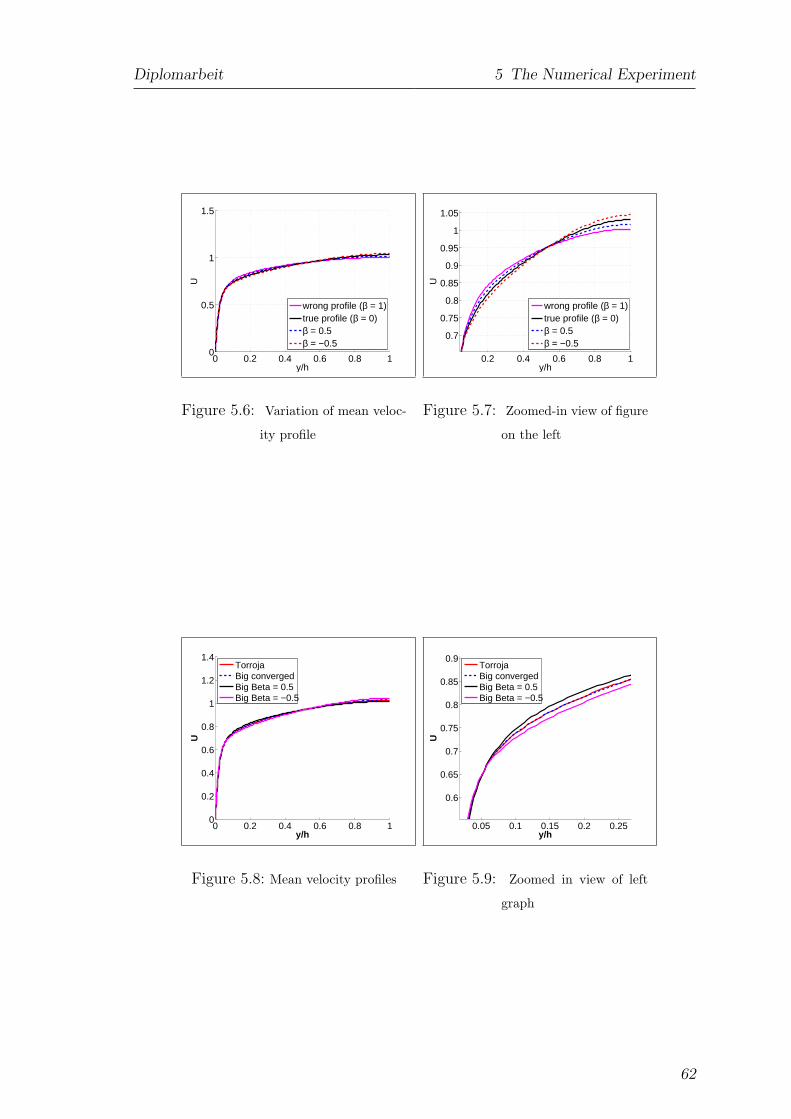
Diplomarbeit 5 The Numerical Experiment
0 0.2 0.4 0.6 0.8 10
0.5
1
1.5
y/h
U
wrong profile (β = 1)true profile (β = 0)β = 0.5β = −0.5
Figure 5.6: Variation of mean veloc-
ity profile
0.2 0.4 0.6 0.8 1
0.7
0.75
0.8
0.85
0.9
0.95
1
1.05
y/h
U
wrong profile (β = 1)true profile (β = 0)β = 0.5β = −0.5
Figure 5.7: Zoomed-in view of figure
on the left
0 0.2 0.4 0.6 0.8 10
0.2
0.4
0.6
0.8
1
1.2
1.4
U
y/h
TorrojaBig convergedBig Beta = 0.5Big Beta = −0.5
Figure 5.8: Mean velocity profiles
0.05 0.1 0.15 0.2 0.25
0.6
0.65
0.7
0.75
0.8
0.85
0.9
U
y/h
TorrojaBig convergedBig Beta = 0.5Big Beta = −0.5
Figure 5.9: Zoomed in view of left
graph
62
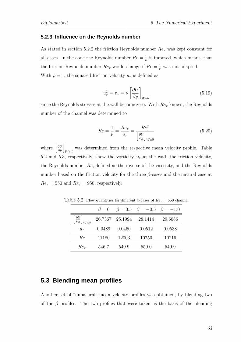
Diplomarbeit 5 The Numerical Experiment
5.2.3 Influence on the Reynolds number
As stated in section 5.2.2 the friction Reynolds number Reτ was kept constant for
all cases. In the code the Reynolds number Re = 1ν
is imposed, which means, that
the friction Reynolds number Reτ would change if Re = 1ν
was not adapted.
With ρ = 1, the squared friction velocity uτ is defined as
u2τ = τw = ν
[
∂U
∂y
]
Wall
(5.19)
since the Reynolds stresses at the wall become zero. With Reτ known, the Reynolds
number of the channel was determined to
Re =1
ν=
Reτ
uτ
=Re2
τ[
∂U∂y
]
Wall
(5.20)
where[
∂U∂y
]
Wallwas determined from the respective mean velocity profile. Table
5.2 and 5.3, respectively, show the vorticity ωz at the wall, the friction velocity,
the Reynolds number Re, defined as the inverse of the viscosity, and the Reynolds
number based on the friction velocity for the three β-cases and the natural case at
Reτ = 550 and Reτ = 950, respectively.
Table 5.2: Flow quantities for different β-cases of Reτ = 550 channel
β = 0 β = 0.5 β = −0.5 β = −1.0[
∂U∂y
]
Wall26.7367 25.1994 28.1414 29.6086
uτ 0.0489 0.0460 0.0512 0.0538
Re 11180 12003 10750 10216
Reτ 546.7 549.9 550.0 549.9
5.3 Blending mean profiles
Another set of “unnatural” mean velocity profiles was obtained, by blending two
of the β profiles. The two profiles that were taken as the basis of the blending
63
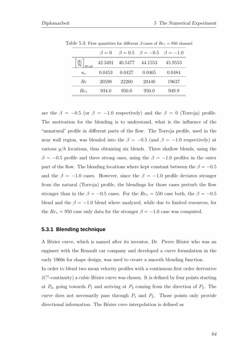
Diplomarbeit 5 The Numerical Experiment
Table 5.3: Flow quantities for different β-cases of Reτ = 950 channel
β = 0 β = 0.5 β = −0.5 β = −1.0[
∂U∂y
]
Wall42.3491 40.5477 44.1553 45.9553
uτ 0.0453 0.0427 0.0465 0.0484
Re 20598 22260 20440 19637
Reτ 934.0 950.0 950.0 949.9
are the β = −0.5 (or β = −1.0 respectively) and the β = 0 (Torroja) profile.
The motivation for the blending is to understand, what is the influence of the
“unnatural” profile in different parts of the flow. The Torroja profile, used in the
near wall region, was blended into the β = −0.5 (and β = −1.0 respectively) at
various y/h locations, thus obtaining six blends. Three shallow blends, using the
β = −0.5 profile and three strong ones, using the β = −1.0 profiles in the outer
part of the flow. The blending locations where kept constant between the β = −0.5
and the β = −1.0 cases. However, since the β = −1.0 profile deviates stronger
from the natural (Torroja) profile, the blendings for those cases perturb the flow
stronger than in the β = −0.5 cases. For the Reτ = 550 case both, the β = −0.5
blend and the β = −1.0 blend where analyzed, while due to limited resources, for
the Reτ = 950 case only data for the stronger β = −1.0 case was computed.
5.3.1 Blending technique
A Bezier curve, which is named after its inventor, Dr. Pierre Bezier who was an
engineer with the Renault car company and developed a curve formulation in the
early 1960s for shape design, was used to create a smooth blending function.
In order to blend two mean velocity profiles with a continuous first order derivative
(C1-continuity) a cubic Bezier curve was chosen. It is defined by four points starting
at P0, going towards P1 and arriving at P3 coming from the direction of P2. The
curve does not necessarily pass through P1 and P2. Those points only provide
directional information. The Bezier cuve interpolation is defined as
64
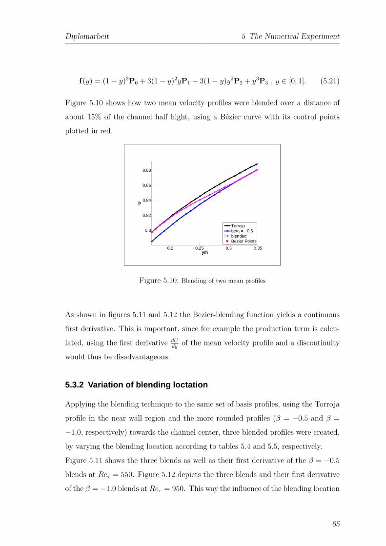
Diplomarbeit 5 The Numerical Experiment
f(y) = (1 − y)3P0 + 3(1 − y)2yP1 + 3(1 − y)y2
P2 + y3P3 , y ∈ [0, 1]. (5.21)
Figure 5.10 shows how two mean velocity profiles were blended over a distance of
about 15% of the channel half hight, using a Bezier curve with its control points
plotted in red.
0.2 0.25 0.3 0.35
0.8
0.82
0.84
0.86
0.88
U
y/h
Torrojabeta = −0.5blendedBezier Points
Figure 5.10: Blending of two mean profiles
As shown in figures 5.11 and 5.12 the Bezier-blending function yields a continuous
first derivative. This is important, since for example the production term is calcu-
lated, using the first derivative dUdy
of the mean velocity profile and a discontinuity
would thus be disadvantageous.
5.3.2 Variation of blending loctation
Applying the blending technique to the same set of basis profiles, using the Torroja
profile in the near wall region and the more rounded profiles (β = −0.5 and β =
−1.0, respectively) towards the channel center, three blended profiles were created,
by varying the blending location according to tables 5.4 and 5.5, respectively.
Figure 5.11 shows the three blends as well as their first derivative of the β = −0.5
blends at Reτ = 550. Figure 5.12 depicts the three blends and their first derivative
of the β = −1.0 blends at Reτ = 950. This way the influence of the blending location
65
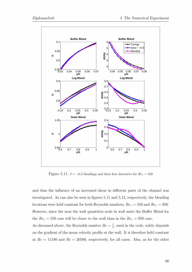
Diplomarbeit 5 The Numerical Experiment
0.03 0.04 0.05 0.06 0.070.55
0.6
0.65
0.7
U
y/h
Buffer Blend
0.04 0.05 0.06 0.07 0.08
2
3
4
5
6
dU/d
y
y/h
Buffer Blend
0.15 0.2 0.25 0.3 0.35
0.8
0.85
0.9
U
y/h
Log Blend
0.15 0.2 0.25 0.3 0.350.3
0.4
0.5
0.6
0.7
0.8
dU/d
y
y/h
Log Blend
0.6 0.7 0.8 0.9 10.95
1
1.05
U
y/h
Outer Blend
0.6 0.7 0.8 0.9 10
0.1
0.2
0.3
0.4
dU/d
y
y/h
Outer Blend
Torrojabeta = −0.5blended
Figure 5.11: β = −0.5 blendings and their first derivative for Reτ = 550
and thus the influence of an increased shear in different parts of the channel was
investigated. As can also be seen in figures 5.11 and 5.12, respectively, the blending
locations were held constant for both Reynolds numbers, Reτ = 550 and Reτ = 950.
However, since the near the wall quantities scale in wall units the Buffer Blend for
the Reτ = 550 case will be closer to the wall than in the Reτ = 950 case.
As discussed above, the Reynolds number Re = 1ν, used in the code, solely depends
on the gradient of the mean velocity profile at the wall. It is therefore held constant
at Re = 11180 and Re = 20580, respectively, for all cases. Also, as for the other
66
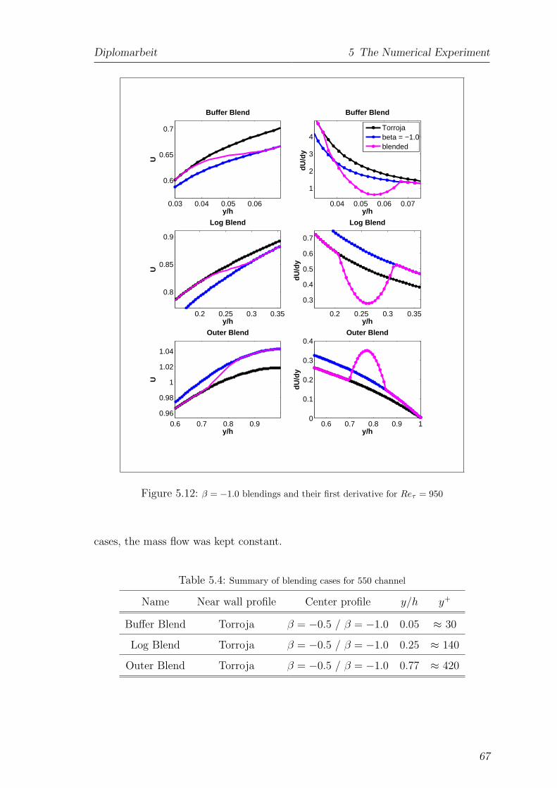
Diplomarbeit 5 The Numerical Experiment
0.03 0.04 0.05 0.06
0.6
0.65
0.7
U
y/h
Buffer Blend
0.04 0.05 0.06 0.07
1
2
3
4
dU/d
y
y/h
Buffer Blend
0.2 0.25 0.3 0.35
0.8
0.85
0.9
U
y/h
Log Blend
0.2 0.25 0.3 0.35
0.3
0.4
0.5
0.6
0.7
dU/d
y
y/h
Log Blend
0.6 0.7 0.8 0.90.96
0.98
1
1.02
1.04
U
y/h
Outer Blend
0.6 0.7 0.8 0.9 10
0.1
0.2
0.3
0.4
dU/d
y
y/h
Outer Blend
Torrojabeta = −1.0blended
Figure 5.12: β = −1.0 blendings and their first derivative for Reτ = 950
cases, the mass flow was kept constant.
Table 5.4: Summary of blending cases for 550 channel
Name Near wall profile Center profile y/h y+
Buffer Blend Torroja β = −0.5 / β = −1.0 0.05 ≈ 30
Log Blend Torroja β = −0.5 / β = −1.0 0.25 ≈ 140
Outer Blend Torroja β = −0.5 / β = −1.0 0.77 ≈ 420
67

Diplomarbeit 5 The Numerical Experiment
Table 5.5: Summary of blending cases for 950 channel
Name Near wall profile Center profile y/h y+
Buffer Blend Torroja β = −1.0 0.05 ≈ 50
Log Blend Torroja β = −1.0 0.25 ≈ 240
Outer Blend Torroja β = −1.0 0.77 ≈ 730
68
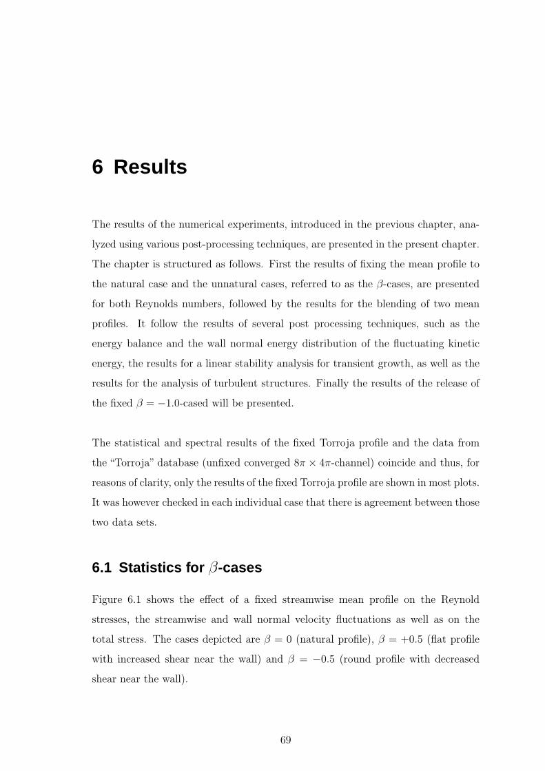
6 Results
The results of the numerical experiments, introduced in the previous chapter, ana-
lyzed using various post-processing techniques, are presented in the present chapter.
The chapter is structured as follows. First the results of fixing the mean profile to
the natural case and the unnatural cases, referred to as the β-cases, are presented
for both Reynolds numbers, followed by the results for the blending of two mean
profiles. It follow the results of several post processing techniques, such as the
energy balance and the wall normal energy distribution of the fluctuating kinetic
energy, the results for a linear stability analysis for transient growth, as well as the
results for the analysis of turbulent structures. Finally the results of the release of
the fixed β = −1.0-cased will be presented.
The statistical and spectral results of the fixed Torroja profile and the data from
the “Torroja” database (unfixed converged 8π × 4π-channel) coincide and thus, for
reasons of clarity, only the results of the fixed Torroja profile are shown in most plots.
It was however checked in each individual case that there is agreement between those
two data sets.
6.1 Statistics for β-cases
Figure 6.1 shows the effect of a fixed streamwise mean profile on the Reynold
stresses, the streamwise and wall normal velocity fluctuations as well as on the
total stress. The cases depicted are β = 0 (natural profile), β = +0.5 (flat profile
with increased shear near the wall) and β = −0.5 (round profile with decreased
shear near the wall).
69
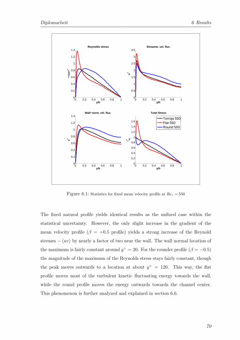
Diplomarbeit 6 Results
0 0.2 0.4 0.6 0.8 10
0.2
0.4
0.6
0.8
1
1.2
1.4
−<uv
>+
y/h
Reynolds stress
0 0.2 0.4 0.6 0.8 10
0.5
1
1.5
2
2.5
3
3.5
u+
y/h
Streamw. vel. fluc.
0 0.2 0.4 0.6 0.8 10
0.2
0.4
0.6
0.8
1
1.2
1.4
v+
y/h
Wall−norm. vel. fluc.
0 0.2 0.4 0.6 0.8 10
0.2
0.4
0.6
0.8
1
1.2
1.4
1.6
τ xy+
y/h
Total Stress
Torroja 550Flat 550Round 550
Figure 6.1: Statistics for fixed mean velocity profile at Reτ = 550
The fixed natural profile yields identical results as the unfixed case within the
statistical uncertainty. However, the only slight increase in the gradient of the
mean velocity profile (β = +0.5 profile) yields a strong increase of the Reynold
stresses −〈uv〉 by nearly a factor of two near the wall. The wall normal location of
the maximum is fairly constant around y+ = 20. For the rounder profile (β = −0.5)
the magnitude of the maximum of the Reynolds stress stays fairly constant, though
the peak moves outwards to a location at about y+ = 120. This way, the flat
profile moves most of the turbulent kinetic fluctuating energy towards the wall,
while the round profile moves the energy outwards towards the channel center.
This phenomenon is further analyzed and explained in section 6.6.
70
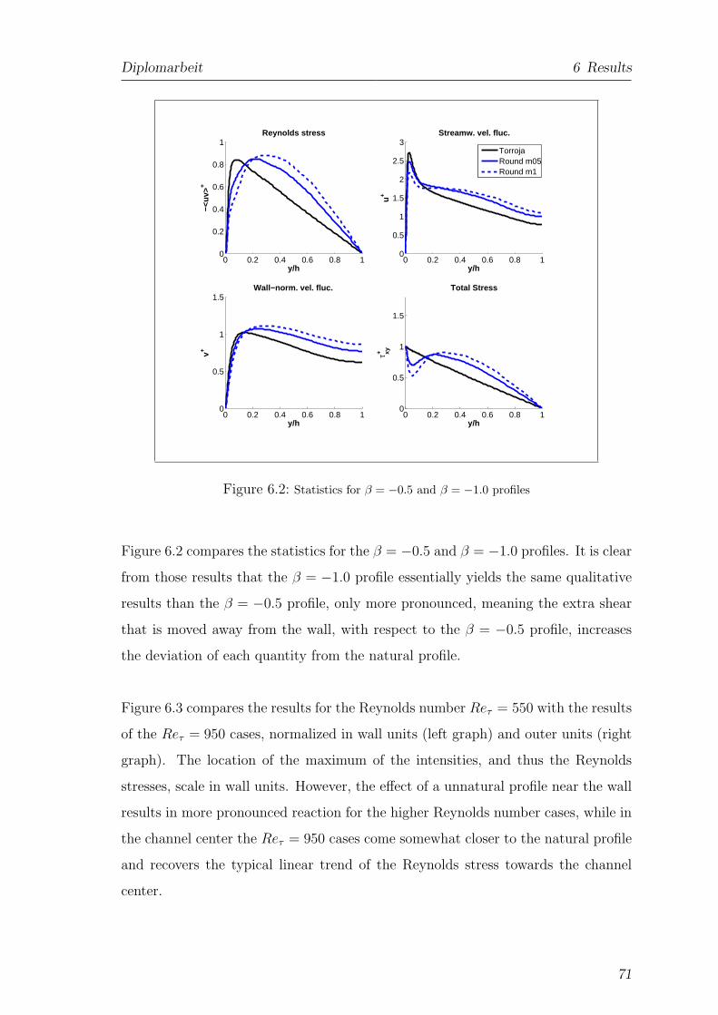
Diplomarbeit 6 Results
0 0.2 0.4 0.6 0.8 10
0.2
0.4
0.6
0.8
1
−<uv
>+
y/h
Reynolds stress
0 0.2 0.4 0.6 0.8 10
0.5
1
1.5
2
2.5
3
u+
y/h
Streamw. vel. fluc.
0 0.2 0.4 0.6 0.8 10
0.5
1
1.5
v+
y/h
Wall−norm. vel. fluc.
0 0.2 0.4 0.6 0.8 10
0.5
1
1.5
τ xy+
y/h
Total Stress
TorrojaRound m05Round m1
Figure 6.2: Statistics for β = −0.5 and β = −1.0 profiles
Figure 6.2 compares the statistics for the β = −0.5 and β = −1.0 profiles. It is clear
from those results that the β = −1.0 profile essentially yields the same qualitative
results than the β = −0.5 profile, only more pronounced, meaning the extra shear
that is moved away from the wall, with respect to the β = −0.5 profile, increases
the deviation of each quantity from the natural profile.
Figure 6.3 compares the results for the Reynolds number Reτ = 550 with the results
of the Reτ = 950 cases, normalized in wall units (left graph) and outer units (right
graph). The location of the maximum of the intensities, and thus the Reynolds
stresses, scale in wall units. However, the effect of a unnatural profile near the wall
results in more pronounced reaction for the higher Reynolds number cases, while in
the channel center the Reτ = 950 cases come somewhat closer to the natural profile
and recovers the typical linear trend of the Reynolds stress towards the channel
center.
71
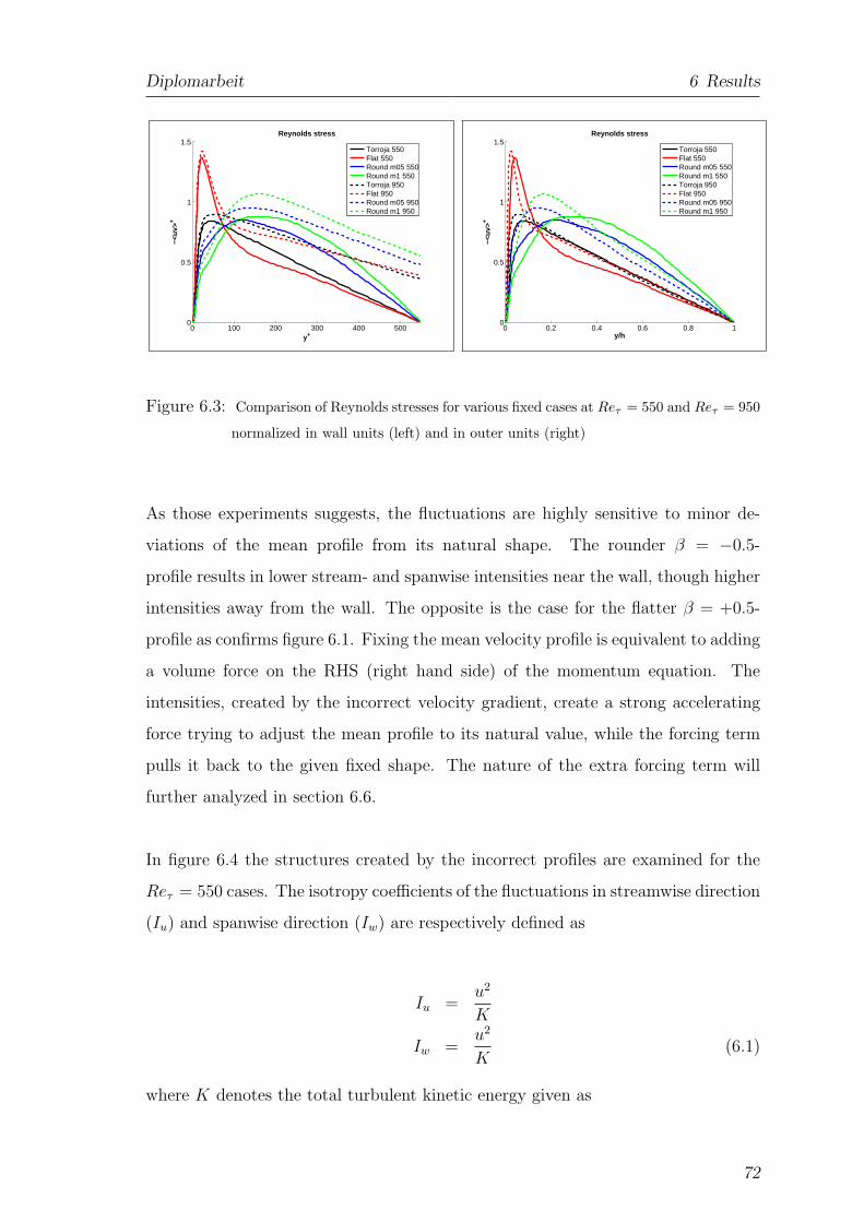
Diplomarbeit 6 Results
0 100 200 300 400 5000
0.5
1
1.5
−<uv
>+
y+
Reynolds stress
Torroja 550Flat 550Round m05 550Round m1 550Torroja 950Flat 950Round m05 950Round m1 950
0 0.2 0.4 0.6 0.8 10
0.5
1
1.5
−<uv
>+
y/h
Reynolds stress
Torroja 550Flat 550Round m05 550Round m1 550Torroja 950Flat 950Round m05 950Round m1 950
Figure 6.3: Comparison of Reynolds stresses for various fixed cases at Reτ = 550 and Reτ = 950
normalized in wall units (left) and in outer units (right)
As those experiments suggests, the fluctuations are highly sensitive to minor de-
viations of the mean profile from its natural shape. The rounder β = −0.5-
profile results in lower stream- and spanwise intensities near the wall, though higher
intensities away from the wall. The opposite is the case for the flatter β = +0.5-
profile as confirms figure 6.1. Fixing the mean velocity profile is equivalent to adding
a volume force on the RHS (right hand side) of the momentum equation. The
intensities, created by the incorrect velocity gradient, create a strong accelerating
force trying to adjust the mean profile to its natural value, while the forcing term
pulls it back to the given fixed shape. The nature of the extra forcing term will
further analyzed in section 6.6.
In figure 6.4 the structures created by the incorrect profiles are examined for the
Reτ = 550 cases. The isotropy coefficients of the fluctuations in streamwise direction
(Iu) and spanwise direction (Iw) are respectively defined as
Iu =u2
K
Iw =u2
K(6.1)
where K denotes the total turbulent kinetic energy given as
72
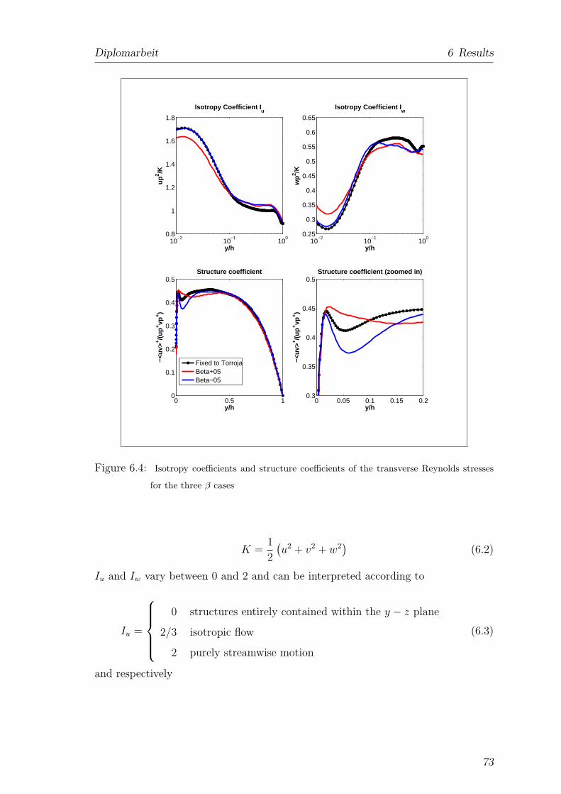
Diplomarbeit 6 Results
10−2
10−1
100
0.8
1
1.2
1.4
1.6
1.8
up2 /K
y/h
Isotropy Coefficient Iu
10−2
10−1
100
0.25
0.3
0.35
0.4
0.45
0.5
0.55
0.6
0.65
wp
2 /K
y/h
Isotropy Coefficient Iw
0 0.5 10
0.1
0.2
0.3
0.4
0.5
−<uv
>+ /(
up+ vp
+ )
y/h
Structure coefficient
0 0.05 0.1 0.15 0.20.3
0.35
0.4
0.45
0.5
−<uv
>+ /(
up+ vp
+ )
y/h
Structure coefficient (zoomed in)
Fixed to TorrojaBeta+05Beta−05
Figure 6.4: Isotropy coefficients and structure coefficients of the transverse Reynolds stresses
for the three β cases
K =1
2
(
u2 + v2 + w2)
(6.2)
Iu and Iw vary between 0 and 2 and can be interpreted according to
Iu =
0 structures entirely contained within the y − z plane
2/3 isotropic flow
2 purely streamwise motion
(6.3)
and respectively
73
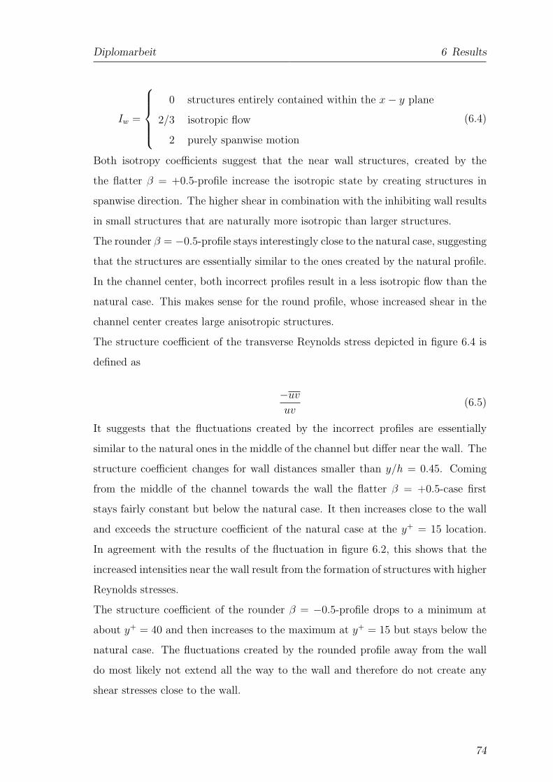
Diplomarbeit 6 Results
Iw =
0 structures entirely contained within the x − y plane
2/3 isotropic flow
2 purely spanwise motion
(6.4)
Both isotropy coefficients suggest that the near wall structures, created by the
the flatter β = +0.5-profile increase the isotropic state by creating structures in
spanwise direction. The higher shear in combination with the inhibiting wall results
in small structures that are naturally more isotropic than larger structures.
The rounder β = −0.5-profile stays interestingly close to the natural case, suggesting
that the structures are essentially similar to the ones created by the natural profile.
In the channel center, both incorrect profiles result in a less isotropic flow than the
natural case. This makes sense for the round profile, whose increased shear in the
channel center creates large anisotropic structures.
The structure coefficient of the transverse Reynolds stress depicted in figure 6.4 is
defined as
−uv
uv(6.5)
It suggests that the fluctuations created by the incorrect profiles are essentially
similar to the natural ones in the middle of the channel but differ near the wall. The
structure coefficient changes for wall distances smaller than y/h = 0.45. Coming
from the middle of the channel towards the wall the flatter β = +0.5-case first
stays fairly constant but below the natural case. It then increases close to the wall
and exceeds the structure coefficient of the natural case at the y+ = 15 location.
In agreement with the results of the fluctuation in figure 6.2, this shows that the
increased intensities near the wall result from the formation of structures with higher
Reynolds stresses.
The structure coefficient of the rounder β = −0.5-profile drops to a minimum at
about y+ = 40 and then increases to the maximum at y+ = 15 but stays below the
natural case. The fluctuations created by the rounded profile away from the wall
do most likely not extend all the way to the wall and therefore do not create any
shear stresses close to the wall.
74
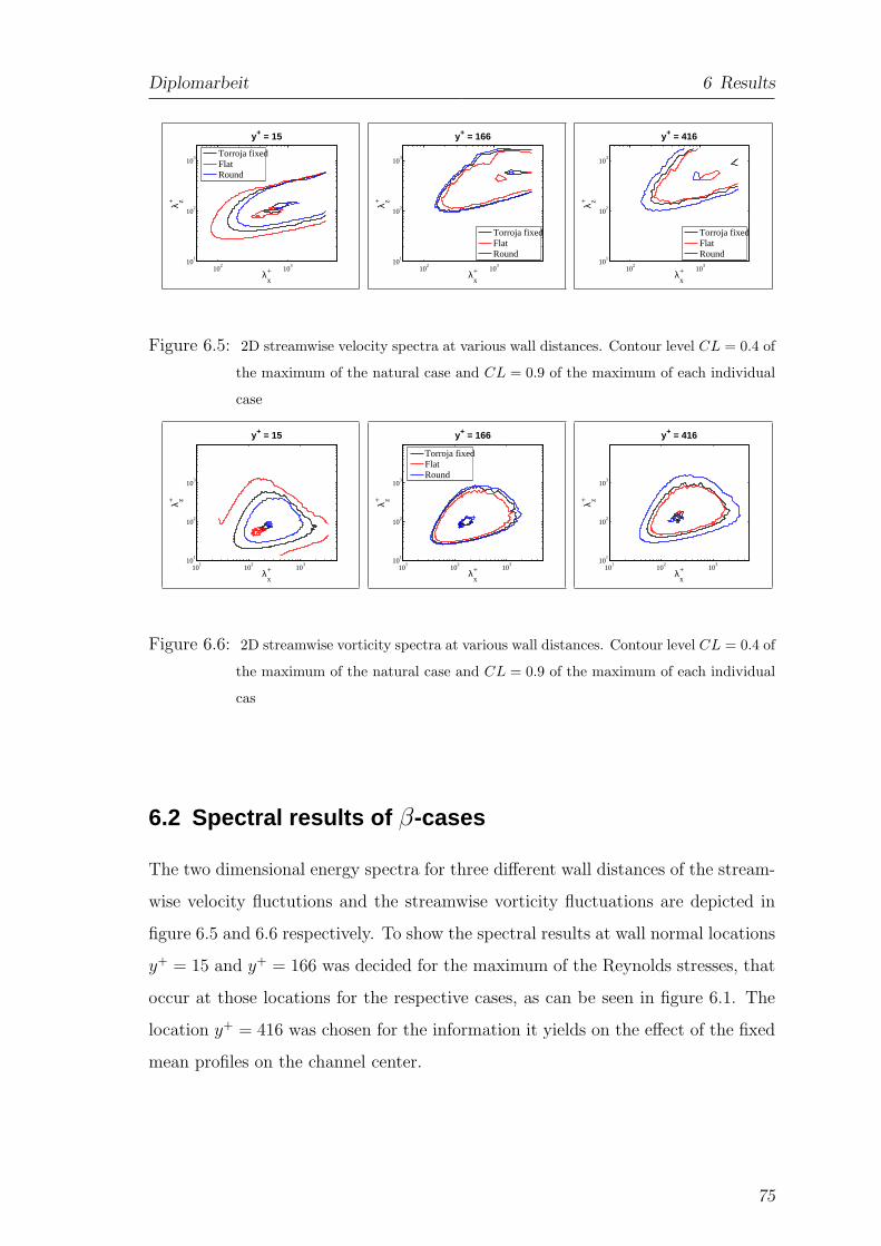
Diplomarbeit 6 Results
102
103
101
102
103
y+ = 15
λ+x
λ+ z
Torroja fixedFlatRound
102
103
101
102
103
y+ = 166
λ+x
λ+ z
Torroja fixedFlatRound
102
103
101
102
103
y+ = 416
λ+x
λ+ z
Torroja fixedFlatRound
Figure 6.5: 2D streamwise velocity spectra at various wall distances. Contour level CL = 0.4 of
the maximum of the natural case and CL = 0.9 of the maximum of each individual
case
101
102
103
101
102
103
y+ = 15
λ+x
λ+ z
101
102
103
101
102
103
y+ = 166
λ+x
λ+ z
Torroja fixedFlatRound
101
102
103
101
102
103
y+ = 416
λ+x
λ+ z
Figure 6.6: 2D streamwise vorticity spectra at various wall distances. Contour level CL = 0.4 of
the maximum of the natural case and CL = 0.9 of the maximum of each individual
cas
6.2 Spectral results of β-cases
The two dimensional energy spectra for three different wall distances of the stream-
wise velocity fluctutions and the streamwise vorticity fluctuations are depicted in
figure 6.5 and 6.6 respectively. To show the spectral results at wall normal locations
y+ = 15 and y+ = 166 was decided for the maximum of the Reynolds stresses, that
occur at those locations for the respective cases, as can be seen in figure 6.1. The
location y+ = 416 was chosen for the information it yields on the effect of the fixed
mean profiles on the channel center.
75
Diplomarbeit 6 Results
As already mentioned above, changing the mean profile changes the size of the
structures that are created. For the flat profile, where the shear is moved towards
the wall, the near wall structures (y+ = 15) become narrower, shorter and about 50%
more intense. This is true for all three velocity spectra (only streamwise direction
shown here). For the round profile, in agreement with the statistics results, the
structures near the wall become less intense and the energy is moved away from the
wall towards the channel center at y+ = 416, where the energy increases in all three
velocity components with respect to the natural case. As show the contour levels
(CL = 0.9) near the peak of the respective spectrum, the entire spectrum is not
distorted but completely shifted.
Interestingly the influence of changing the mean profile does not only effect the
large scale structures but changes the small scale structures (such as vorticity) in
the same manner. Figure 6.6 shows the two dimensional energy spectrum of the
streamwise vorticity. Just like the large scale fluctuations of the velocities, the
vorticity fluctuations get more intense near the wall for the flat profile while energy
is added by the round profile in the channel center. This indicates that by changing
the mean shear not only structures of similar sizes, but structures at both ends of
the cascade are affected in the same manner, suggesting that the energy, that is fed
into the large scales by the mean shear is passed down the self similar cascade locally.
Figure 6.7 shows the pre-multiplied kinetic energy spectra splitted up into its three
components for the same three wall distances y+ = 15, y+ = 166 and y+ = 416 for
the three β-cases: Natural, flat and round.
Near the wall (y+ = 15), the wave number κ of the maximum of the flat profile
increases for all three components suggesting that most of the additional energy, that
is created near the wall, is added to the smaller scales (higher wave numbers) than in
the natural case. The largest increase in terms of the wave number can be observed
in the spanwise direction. Also, the relative increase of the extra energy added is
about 50% larger in spanwise and wall normal direction where the energy doubles
with respect to the natural case. In streamwise direction the energy increases only
76
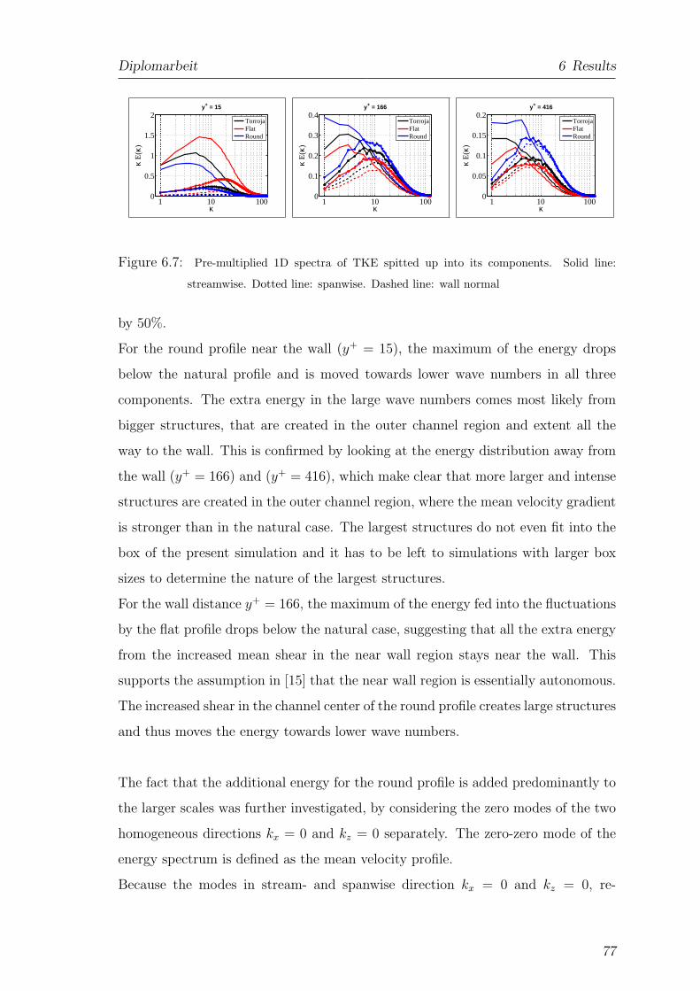
Diplomarbeit 6 Results
1 10 1000
0.5
1
1.5
2y+ = 15
κ
κ E
(κ)
TorrojaFlatRound
1 10 1000
0.1
0.2
0.3
0.4y+ = 166
κ
κ E
(κ)
TorrojaFlatRound
1 10 1000
0.05
0.1
0.15
0.2y+ = 416
κ
κ E
(κ)
TorrojaFlatRound
Figure 6.7: Pre-multiplied 1D spectra of TKE spitted up into its components. Solid line:
streamwise. Dotted line: spanwise. Dashed line: wall normal
by 50%.
For the round profile near the wall (y+ = 15), the maximum of the energy drops
below the natural profile and is moved towards lower wave numbers in all three
components. The extra energy in the large wave numbers comes most likely from
bigger structures, that are created in the outer channel region and extent all the
way to the wall. This is confirmed by looking at the energy distribution away from
the wall (y+ = 166) and (y+ = 416), which make clear that more larger and intense
structures are created in the outer channel region, where the mean velocity gradient
is stronger than in the natural case. The largest structures do not even fit into the
box of the present simulation and it has to be left to simulations with larger box
sizes to determine the nature of the largest structures.
For the wall distance y+ = 166, the maximum of the energy fed into the fluctuations
by the flat profile drops below the natural case, suggesting that all the extra energy
from the increased mean shear in the near wall region stays near the wall. This
supports the assumption in [15] that the near wall region is essentially autonomous.
The increased shear in the channel center of the round profile creates large structures
and thus moves the energy towards lower wave numbers.
The fact that the additional energy for the round profile is added predominantly to
the larger scales was further investigated, by considering the zero modes of the two
homogeneous directions kx = 0 and kz = 0 separately. The zero-zero mode of the
energy spectrum is defined as the mean velocity profile.
Because the modes in stream- and spanwise direction kx = 0 and kz = 0, re-
77
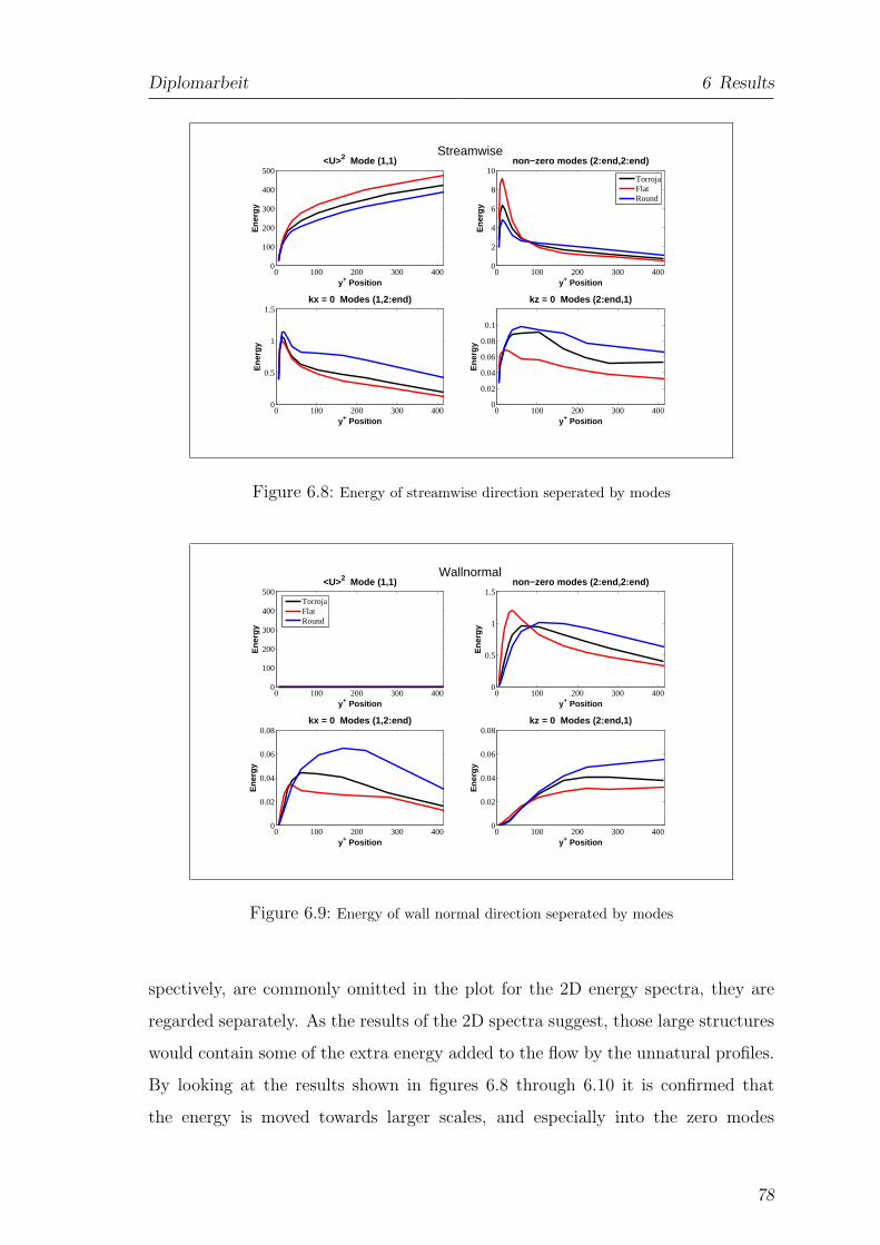
Diplomarbeit 6 Results
Streamwise
0 100 200 300 4000
100
200
300
400
500<U>2 Mode (1,1)
y+ Position
Ene
rgy
0 100 200 300 4000
0.5
1
1.5kx = 0 Modes (1,2:end)
y+ Position
Ene
rgy
0 100 200 300 4000
0.02
0.04
0.06
0.08
0.1
kz = 0 Modes (2:end,1)
y+ Position
Ene
rgy
0 100 200 300 4000
2
4
6
8
10non−zero modes (2:end,2:end)
y+ Position
Ene
rgy
TorrojaFlatRound
Figure 6.8: Energy of streamwise direction seperated by modes
Wallnormal
0 100 200 300 4000
100
200
300
400
500<U>2 Mode (1,1)
y+ Position
Ene
rgy
0 100 200 300 4000
0.02
0.04
0.06
0.08kx = 0 Modes (1,2:end)
y+ Position
Ene
rgy
0 100 200 300 4000
0.02
0.04
0.06
0.08kz = 0 Modes (2:end,1)
y+ Position
Ene
rgy
0 100 200 300 4000
0.5
1
1.5non−zero modes (2:end,2:end)
y+ Position
Ene
rgy
TorrojaFlatRound
Figure 6.9: Energy of wall normal direction seperated by modes
spectively, are commonly omitted in the plot for the 2D energy spectra, they are
regarded separately. As the results of the 2D spectra suggest, those large structures
would contain some of the extra energy added to the flow by the unnatural profiles.
By looking at the results shown in figures 6.8 through 6.10 it is confirmed that
the energy is moved towards larger scales, and especially into the zero modes
78
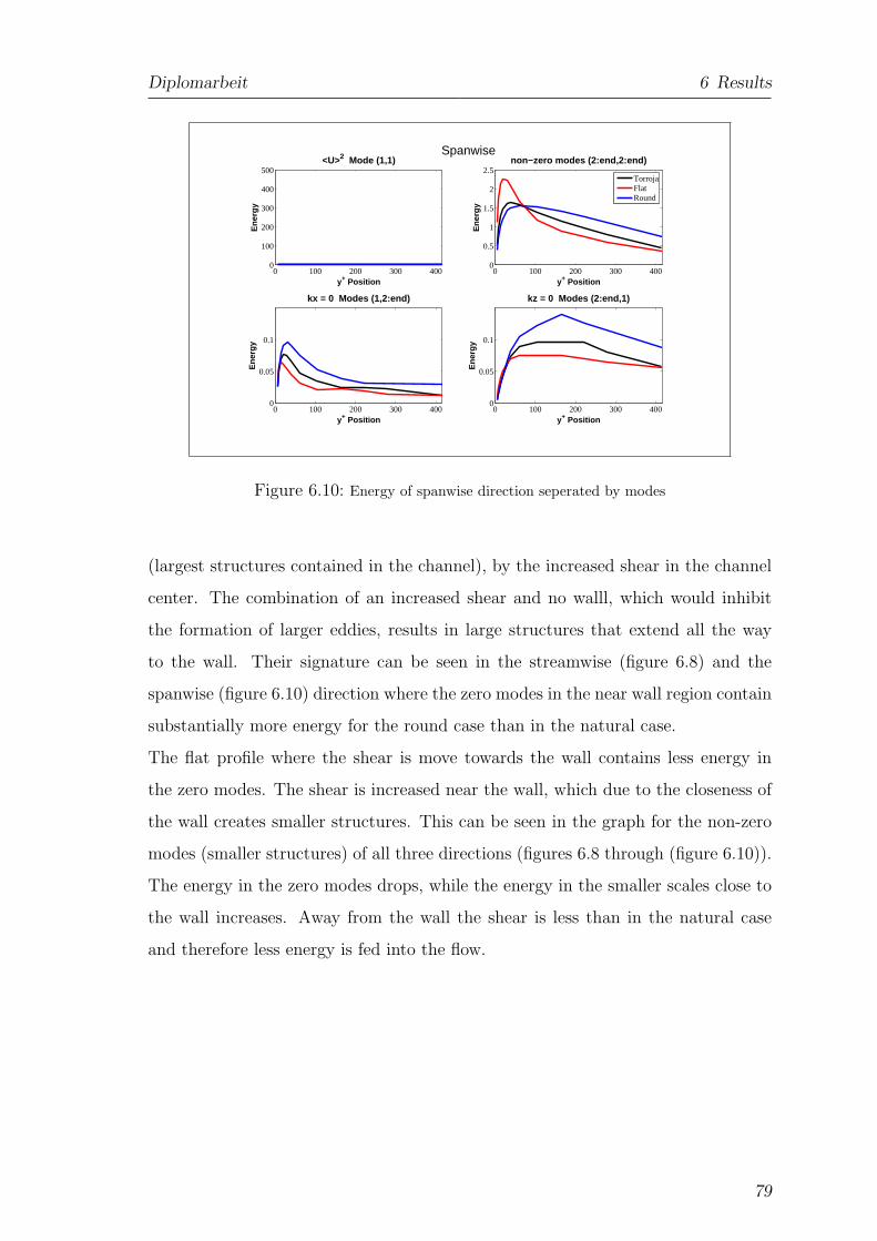
Diplomarbeit 6 Results
Spanwise
0 100 200 300 4000
100
200
300
400
500<U>2 Mode (1,1)
y+ Position
Ene
rgy
0 100 200 300 4000
0.05
0.1
kx = 0 Modes (1,2:end)
y+ Position
Ene
rgy
0 100 200 300 4000
0.05
0.1
kz = 0 Modes (2:end,1)
y+ Position
Ene
rgy
0 100 200 300 4000
0.5
1
1.5
2
2.5non−zero modes (2:end,2:end)
y+ Position
Ene
rgy
TorrojaFlatRound
Figure 6.10: Energy of spanwise direction seperated by modes
(largest structures contained in the channel), by the increased shear in the channel
center. The combination of an increased shear and no walll, which would inhibit
the formation of larger eddies, results in large structures that extend all the way
to the wall. Their signature can be seen in the streamwise (figure 6.8) and the
spanwise (figure 6.10) direction where the zero modes in the near wall region contain
substantially more energy for the round case than in the natural case.
The flat profile where the shear is move towards the wall contains less energy in
the zero modes. The shear is increased near the wall, which due to the closeness of
the wall creates smaller structures. This can be seen in the graph for the non-zero
modes (smaller structures) of all three directions (figures 6.8 through (figure 6.10)).
The energy in the zero modes drops, while the energy in the smaller scales close to
the wall increases. Away from the wall the shear is less than in the natural case
and therefore less energy is fed into the flow.
79
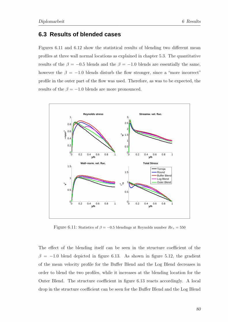
Diplomarbeit 6 Results
6.3 Results of blended cases
Figures 6.11 and 6.12 show the statistical results of blending two different mean
profiles at three wall normal locations as explained in chapter 5.3. The quantitative
results of the β = −0.5 blends and the β = −1.0 blends are essentially the same,
however the β = −1.0 blends disturb the flow stronger, since a “more incorrect”
profile in the outer part of the flow was used. Therefore, as was to be expected, the
results of the β = −1.0 blends are more pronounced.
0 0.2 0.4 0.6 0.8 10
0.2
0.4
0.6
0.8
1
−<uv
>+
y/h
Reynolds stress
0 0.2 0.4 0.6 0.8 10
0.5
1
1.5
2
2.5
3
u+
y/h
Streamw. vel. fluc.
0 0.2 0.4 0.6 0.8 10
0.5
1
1.5
v+
y/h
Wall−norm. vel. fluc.
0 0.2 0.4 0.6 0.8 10
0.5
1
1.5
τ xy+
y/h
Total Stress
TorrojaRoundBuffer BlendLog BlendOuter Blend
Figure 6.11: Statistics of β = −0.5 blendings at Reynolds number Reτ = 550
The effect of the blending itself can be seen in the structure coefficient of the
β = −1.0 blend depicted in figure 6.13. As shown in figure 5.12, the gradient
of the mean velocity profile for the Buffer Blend and the Log Blend decreases in
order to blend the two profiles, while it increases at the blending location for the
Outer Blend. The structure coefficient in figure 6.13 reacts accordingly. A local
drop in the structure coefficient can be seen for the Buffer Blend and the Log Blend
80
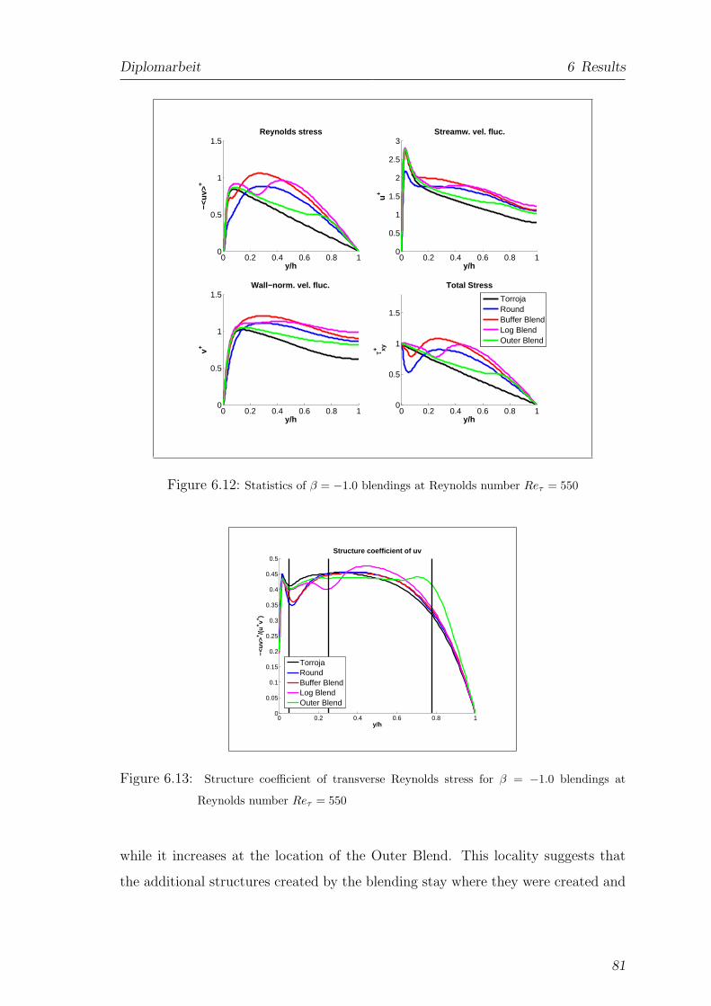
Diplomarbeit 6 Results
0 0.2 0.4 0.6 0.8 10
0.5
1
1.5
−<uv
>+
y/h
Reynolds stress
0 0.2 0.4 0.6 0.8 10
0.5
1
1.5
2
2.5
3
u+
y/h
Streamw. vel. fluc.
0 0.2 0.4 0.6 0.8 10
0.5
1
1.5
v+
y/h
Wall−norm. vel. fluc.
0 0.2 0.4 0.6 0.8 10
0.5
1
1.5
τ xy+
y/h
Total Stress
TorrojaRoundBuffer BlendLog BlendOuter Blend
Figure 6.12: Statistics of β = −1.0 blendings at Reynolds number Reτ = 550
0 0.2 0.4 0.6 0.8 10
0.05
0.1
0.15
0.2
0.25
0.3
0.35
0.4
0.45
0.5
−<uv
>+ /(
u+ v+ )
y/h
Structure coefficient of uv
TorrojaRoundBuffer BlendLog BlendOuter Blend
Figure 6.13: Structure coefficient of transverse Reynolds stress for β = −1.0 blendings at
Reynolds number Reτ = 550
while it increases at the location of the Outer Blend. This locality suggests that
the additional structures created by the blending stay where they were created and
81
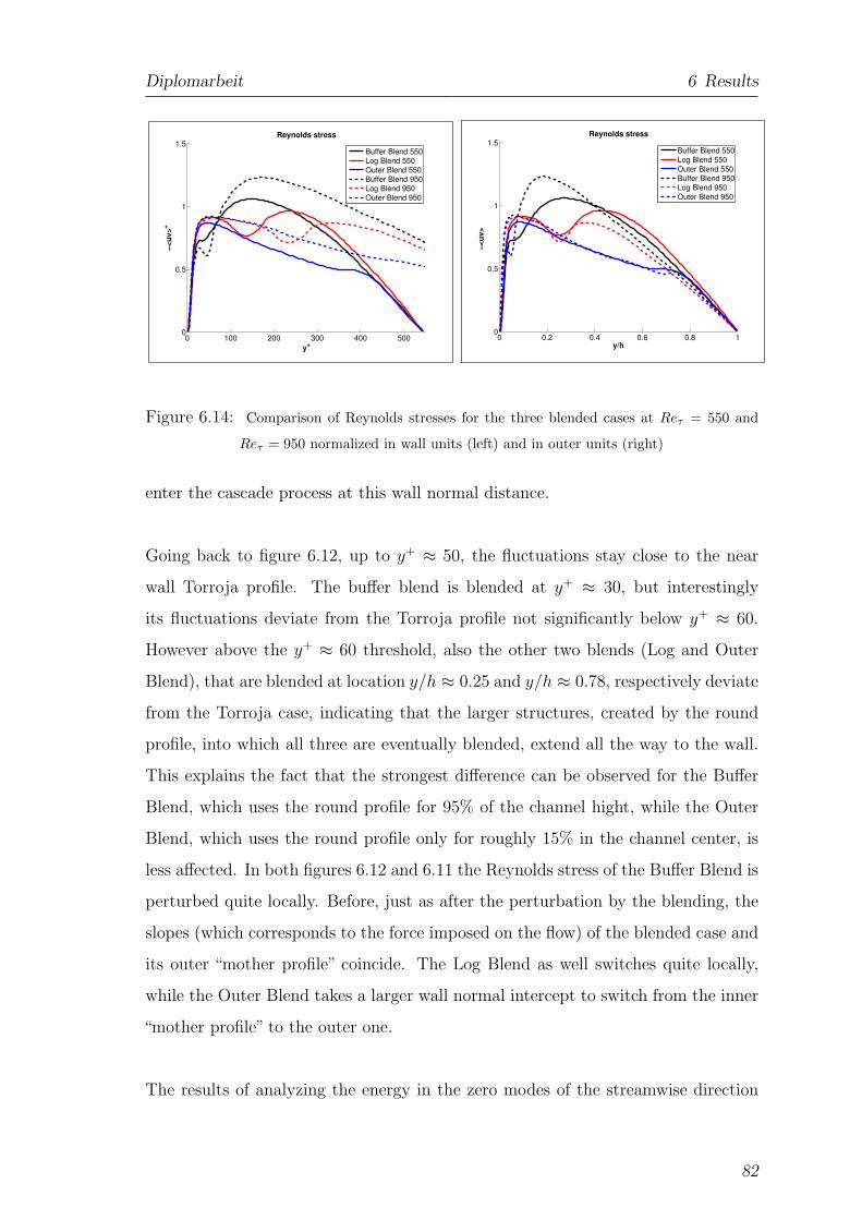
Diplomarbeit 6 Results
0 100 200 300 400 5000
0.5
1
1.5
−<uv>+
y+
Reynolds stress
Buffer Blend 550Log Blend 550Outer Blend 550Buffer Blend 950Log Blend 950Outer Blend 950
0 0.2 0.4 0.6 0.8 10
0.5
1
1.5
−<uv>
y/h
Reynolds stress
Buffer Blend 550Log Blend 550Outer Blend 550Buffer Blend 950Log Blend 950Outer Blend 950
Figure 6.14: Comparison of Reynolds stresses for the three blended cases at Reτ = 550 and
Reτ = 950 normalized in wall units (left) and in outer units (right)
enter the cascade process at this wall normal distance.
Going back to figure 6.12, up to y+ ≈ 50, the fluctuations stay close to the near
wall Torroja profile. The buffer blend is blended at y+ ≈ 30, but interestingly
its fluctuations deviate from the Torroja profile not significantly below y+ ≈ 60.
However above the y+ ≈ 60 threshold, also the other two blends (Log and Outer
Blend), that are blended at location y/h ≈ 0.25 and y/h ≈ 0.78, respectively deviate
from the Torroja case, indicating that the larger structures, created by the round
profile, into which all three are eventually blended, extend all the way to the wall.
This explains the fact that the strongest difference can be observed for the Buffer
Blend, which uses the round profile for 95% of the channel hight, while the Outer
Blend, which uses the round profile only for roughly 15% in the channel center, is
less affected. In both figures 6.12 and 6.11 the Reynolds stress of the Buffer Blend is
perturbed quite locally. Before, just as after the perturbation by the blending, the
slopes (which corresponds to the force imposed on the flow) of the blended case and
its outer “mother profile” coincide. The Log Blend as well switches quite locally,
while the Outer Blend takes a larger wall normal intercept to switch from the inner
“mother profile” to the outer one.
The results of analyzing the energy in the zero modes of the streamwise direction
82
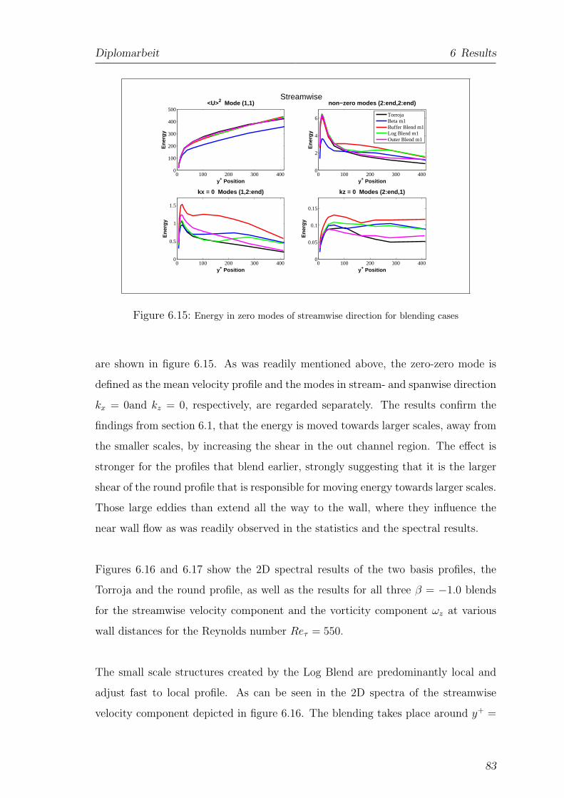
Diplomarbeit 6 Results
Streamwise
0 100 200 300 4000
100
200
300
400
500<U>2 Mode (1,1)
y+ Position
Ene
rgy
0 100 200 300 4000
0.5
1
1.5
kx = 0 Modes (1,2:end)
y+ Position
Ene
rgy
0 100 200 300 4000
0.05
0.1
0.15
kz = 0 Modes (2:end,1)
y+ Position
Ene
rgy
0 100 200 300 4000
2
4
6
non−zero modes (2:end,2:end)
y+ Position
Ene
rgy
TorrojaBeta m1Buffer Blend m1Log Blend m1Outer Blend m1
Figure 6.15: Energy in zero modes of streamwise direction for blending cases
are shown in figure 6.15. As was readily mentioned above, the zero-zero mode is
defined as the mean velocity profile and the modes in stream- and spanwise direction
kx = 0and kz = 0, respectively, are regarded separately. The results confirm the
findings from section 6.1, that the energy is moved towards larger scales, away from
the smaller scales, by increasing the shear in the out channel region. The effect is
stronger for the profiles that blend earlier, strongly suggesting that it is the larger
shear of the round profile that is responsible for moving energy towards larger scales.
Those large eddies than extend all the way to the wall, where they influence the
near wall flow as was readily observed in the statistics and the spectral results.
Figures 6.16 and 6.17 show the 2D spectral results of the two basis profiles, the
Torroja and the round profile, as well as the results for all three β = −1.0 blends
for the streamwise velocity component and the vorticity component ωz at various
wall distances for the Reynolds number Reτ = 550.
The small scale structures created by the Log Blend are predominantly local and
adjust fast to local profile. As can be seen in the 2D spectra of the streamwise
velocity component depicted in figure 6.16. The blending takes place around y+ =
83
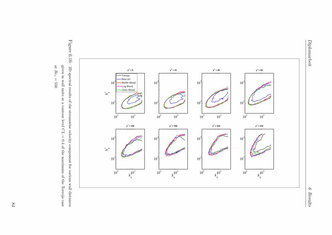
Dip
lom
arb
eit6
Resu
lts
102
103
102
103
y+ = 9
λ+ z
102
103
102
103
y+ = 15
102
103
102
103
y+ = 30
102
103
102
103
y+ = 60
102
103
102
103
y+ = 105
λ+x
λ+ z
102
103
102
103
y+ = 166
λ+x
102
103
102
103
y+ = 222
λ+x
102
103
102
103
y+ = 416
λ+x
TorrojaBeta m1Buffer BlendLog BlendOuter Blend
Figu
re6.16:
2Dsp
ectralresu
ltsof
the
streamw
isevelo
citycom
pon
entfor
various
wall
distan
ces
given
inw
allunits
ata
contou
rlev
elC
L=
0.4of
the
max
imum
ofth
eTorro
jacase
atR
eτ
=550
84
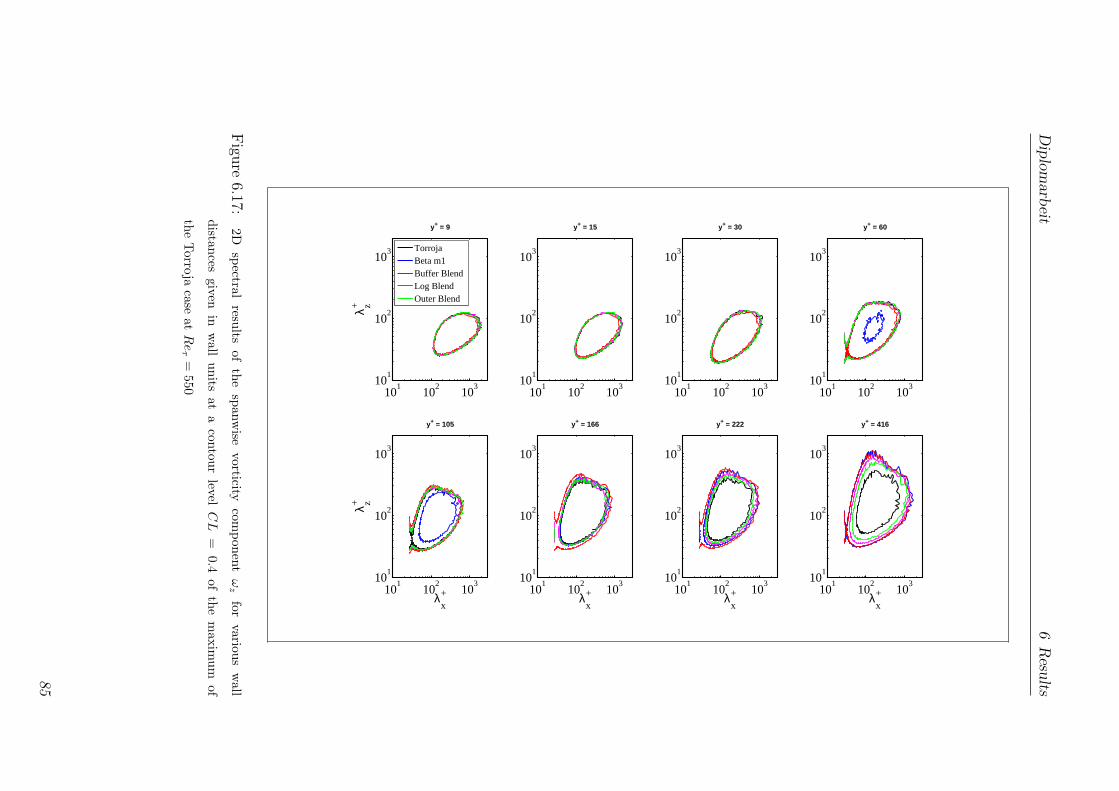
Dip
lom
arb
eit6
Resu
lts
101
102
10310
1
102
103
y+ = 9
λ+ z
101
102
10310
1
102
103
y+ = 15
101
102
10310
1
102
103
y+ = 30
101
102
10310
1
102
103
y+ = 60
101
102
10310
1
102
103
y+ = 105
λ+x
λ+ z
101
102
10310
1
102
103
y+ = 166
λ+x
101
102
10310
1
102
103
y+ = 222
λ+x
101
102
10310
1
102
103
y+ = 416
λ+x
TorrojaBeta m1Buffer BlendLog BlendOuter Blend
Figu
re6.17:
2Dsp
ectralresu
ltsof
the
span
wise
vorticity
compon
ent
ωz
forvariou
sw
all
distan
cesgiv
enin
wall
units
ata
contou
rlev
elC
L=
0.4of
the
max
imum
of
the
Torro
jacase
atR
eτ
=550
85
Diplomarbeit 6 Results
140. The spectrum at y+ = 105 still coincides well with the inner Torroja case,
while the spectrum at y+ = 166 already matches the round β = −1.0 profile into
which it is blended. This suggests that either the small scales have smaller time
scales than the larger structures within which they are contained and thus adapt
faster to the local equilibrium, or the eddies are long and thin without a very big
wall normal extension.
The buffer blend separates much later (y+ ≈ 140) from the near wall Torroja profile
than its blending location (y+ ≈ 30) would suggest. It must be the influence of the
large structures from the channel center that extent all the way to the wall. The
Outer Blend again switches quite locally.
By looking at the large scales (large λx and large λz, respectively) in figure 6.16, it
once more becomes clear that energy is moved towards larger structures by moving
the shear outwards and that all three blends tend towards the round profile even
before the blending has occurred. There is more energy in the large scales for the
blended profiles, explaining where the extra energy moves that was observed in the
Reynolds stress statistics in figure 6.12. The closer to the wall the blending occurs,
the greater is the increase of extra energy in the large scales, confirming that the
round profile increases the amount of energy in the large scales.
That suggests that the mean profile preferably interacts with scales of similar sizes
but since all scales at a given wall distance show the same reaction to a changed mean
profile (see spanwise vorticity component ωz in figure 6.17), it can be assumed that
the cascade process acts locally and faster than the time scale of the large eddies.
6.4 Intersection Point
An interesting observation is the fact, that the profile of the Reynolds stress of the
natural case intersects with the profiles of the Reynolds stresses of the unnatural
cases in one point at y+ ≈ 75, scaled in wall units, and depicted in figure 6.18. This
is true for both Reynolds numbers. Most likely the mean shear and therefore the
86
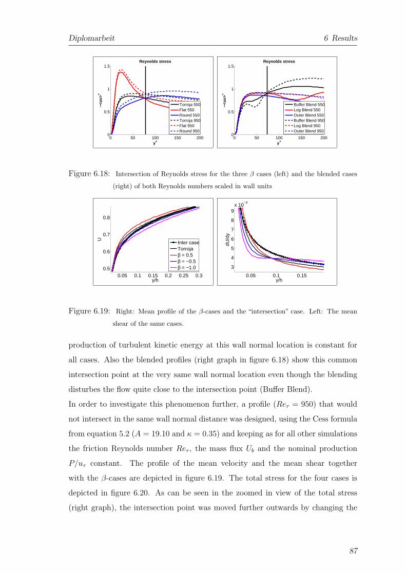
Diplomarbeit 6 Results
0 50 100 150 2000
0.5
1
1.5
−<uv
>+
y+
Reynolds stress
Torroja 550Flat 550Round 550Torroja 950Flat 950Round 950
0 50 100 150 2000
0.5
1
1.5
−<uv
>+
y+
Reynolds stress
Buffer Blend 550Log Blend 550Outer Blend 550Buffer Blend 950Log Blend 950Outer Blend 950
Figure 6.18: Intersection of Reynolds stress for the three β cases (left) and the blended cases
(right) of both Reynolds numbers scaled in wall units
0.05 0.1 0.15 0.2 0.25 0.30.5
0.6
0.7
0.8
y/h
U
Inter caseTorrojaβ = 0.5β = −0.5β = −1.0
0.05 0.1 0.15
3
4
5
6
7
8
9x 10
−3
dU/d
y
y/h
Figure 6.19: Right: Mean profile of the β-cases and the “intersection” case. Left: The mean
shear of the same cases.
production of turbulent kinetic energy at this wall normal location is constant for
all cases. Also the blended profiles (right graph in figure 6.18) show this common
intersection point at the very same wall normal location even though the blending
disturbes the flow quite close to the intersection point (Buffer Blend).
In order to investigate this phenomenon further, a profile (Reτ = 950) that would
not intersect in the same wall normal distance was designed, using the Cess formula
from equation 5.2 (A = 19.10 and κ = 0.35) and keeping as for all other simulations
the friction Reynolds number Reτ , the mass flux Ub and the nominal production
P/uτ constant. The profile of the mean velocity and the mean shear together
with the β-cases are depicted in figure 6.19. The total stress for the four cases is
depicted in figure 6.20. As can be seen in the zoomed in view of the total stress
(right graph), the intersection point was moved further outwards by changing the
87
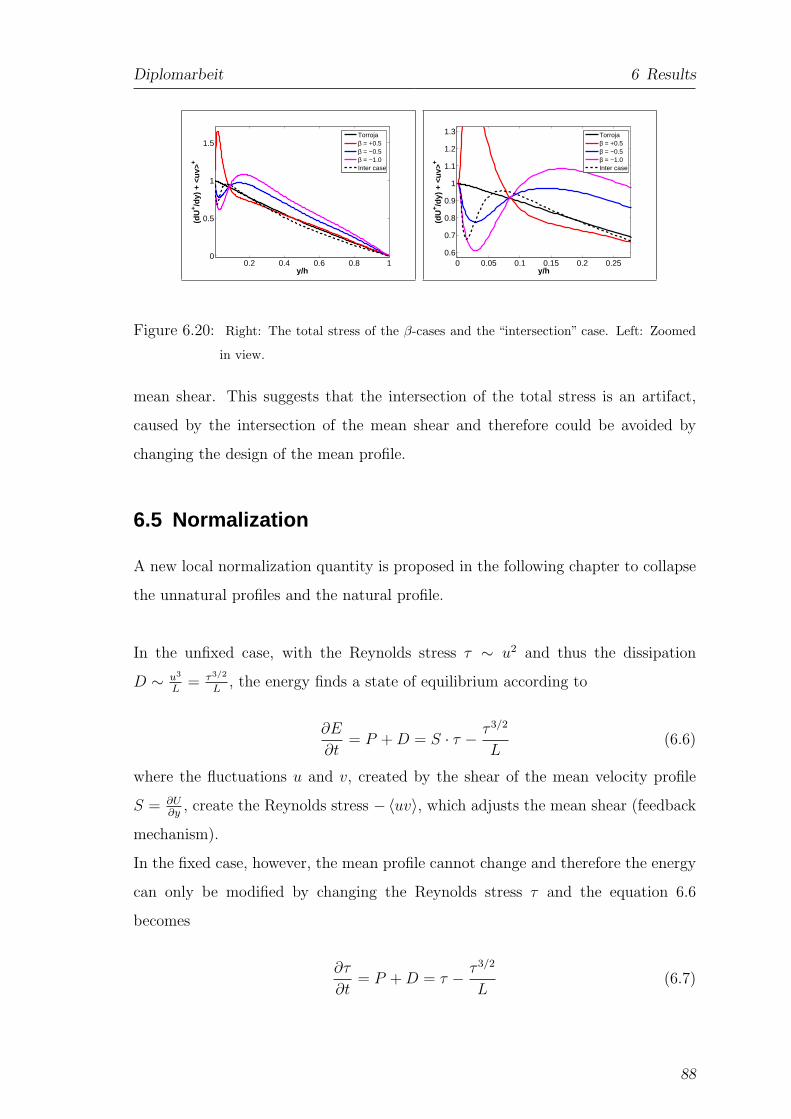
Diplomarbeit 6 Results
0.2 0.4 0.6 0.8 10
0.5
1
1.5
(dU
+ /dy)
+ <
uv>
+
y/h
Torrojaβ = +0.5β = −0.5β = −1.0Inter case
0 0.05 0.1 0.15 0.2 0.250.6
0.7
0.8
0.9
1
1.1
1.2
1.3
(dU
+ /dy)
+ <
uv>
+
y/h
Torrojaβ = +0.5β = −0.5β = −1.0Inter case
Figure 6.20: Right: The total stress of the β-cases and the “intersection” case. Left: Zoomed
in view.
mean shear. This suggests that the intersection of the total stress is an artifact,
caused by the intersection of the mean shear and therefore could be avoided by
changing the design of the mean profile.
6.5 Normalization
A new local normalization quantity is proposed in the following chapter to collapse
the unnatural profiles and the natural profile.
In the unfixed case, with the Reynolds stress τ ∼ u2 and thus the dissipation
D ∼ u3
L= τ3/2
L, the energy finds a state of equilibrium according to
∂E
∂t= P + D = S · τ − τ 3/2
L(6.6)
where the fluctuations u and v, created by the shear of the mean velocity profile
S = ∂U∂y
, create the Reynolds stress −〈uv〉, which adjusts the mean shear (feedback
mechanism).
In the fixed case, however, the mean profile cannot change and therefore the energy
can only be modified by changing the Reynolds stress τ and the equation 6.6
becomes
∂τ
∂t= P + D = τ − τ 3/2
L(6.7)
88
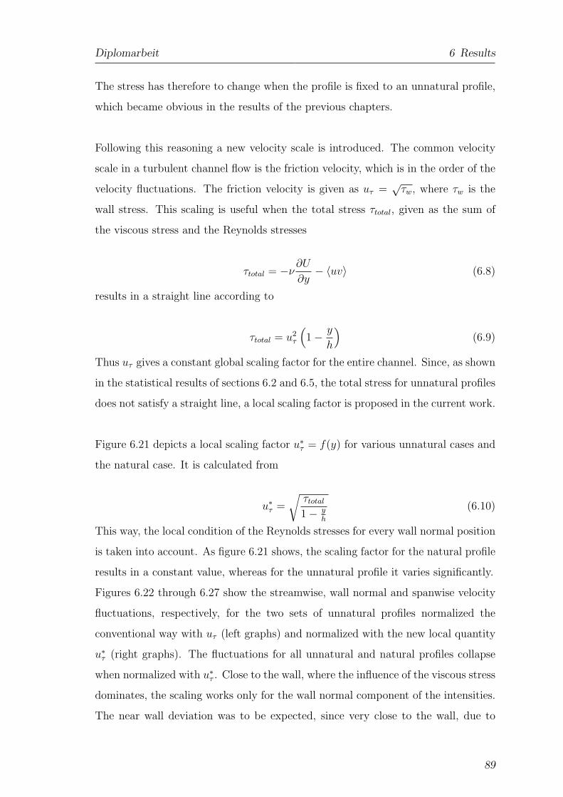
Diplomarbeit 6 Results
The stress has therefore to change when the profile is fixed to an unnatural profile,
which became obvious in the results of the previous chapters.
Following this reasoning a new velocity scale is introduced. The common velocity
scale in a turbulent channel flow is the friction velocity, which is in the order of the
velocity fluctuations. The friction velocity is given as uτ =√
τw, where τw is the
wall stress. This scaling is useful when the total stress τtotal, given as the sum of
the viscous stress and the Reynolds stresses
τtotal = −ν∂U
∂y− 〈uv〉 (6.8)
results in a straight line according to
τtotal = u2τ
(
1 − y
h
)
(6.9)
Thus uτ gives a constant global scaling factor for the entire channel. Since, as shown
in the statistical results of sections 6.2 and 6.5, the total stress for unnatural profiles
does not satisfy a straight line, a local scaling factor is proposed in the current work.
Figure 6.21 depicts a local scaling factor u∗
τ = f(y) for various unnatural cases and
the natural case. It is calculated from
u∗
τ =
√
τtotal
1 − yh
(6.10)
This way, the local condition of the Reynolds stresses for every wall normal position
is taken into account. As figure 6.21 shows, the scaling factor for the natural profile
results in a constant value, whereas for the unnatural profile it varies significantly.
Figures 6.22 through 6.27 show the streamwise, wall normal and spanwise velocity
fluctuations, respectively, for the two sets of unnatural profiles normalized the
conventional way with uτ (left graphs) and normalized with the new local quantity
u∗
τ (right graphs). The fluctuations for all unnatural and natural profiles collapse
when normalized with u∗
τ . Close to the wall, where the influence of the viscous stress
dominates, the scaling works only for the wall normal component of the intensities.
The near wall deviation was to be expected, since very close to the wall, due to
89
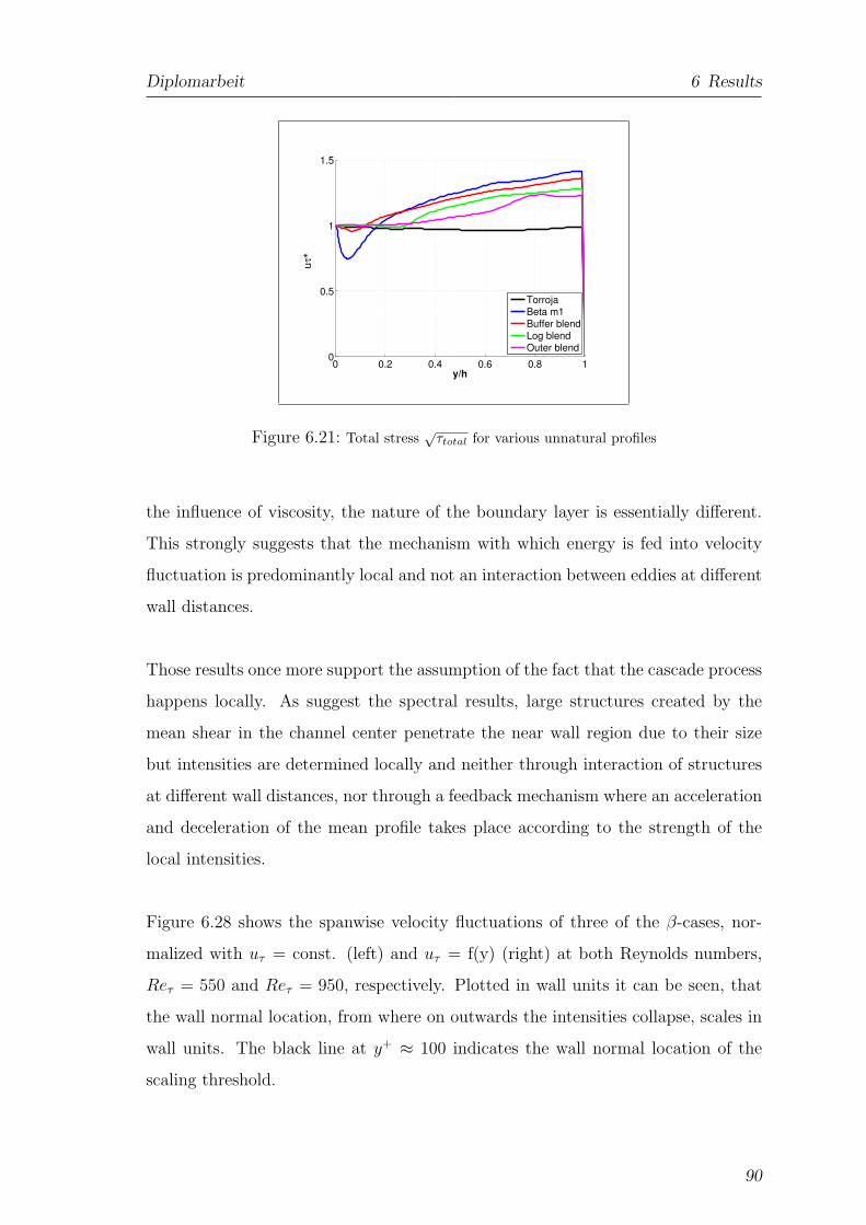
Diplomarbeit 6 Results
Figure 6.21: Total stress√
τtotal for various unnatural profiles
the influence of viscosity, the nature of the boundary layer is essentially different.
This strongly suggests that the mechanism with which energy is fed into velocity
fluctuation is predominantly local and not an interaction between eddies at different
wall distances.
Those results once more support the assumption of the fact that the cascade process
happens locally. As suggest the spectral results, large structures created by the
mean shear in the channel center penetrate the near wall region due to their size
but intensities are determined locally and neither through interaction of structures
at different wall distances, nor through a feedback mechanism where an acceleration
and deceleration of the mean profile takes place according to the strength of the
local intensities.
Figure 6.28 shows the spanwise velocity fluctuations of three of the β-cases, nor-
malized with uτ = const. (left) and uτ = f(y) (right) at both Reynolds numbers,
Reτ = 550 and Reτ = 950, respectively. Plotted in wall units it can be seen, that
the wall normal location, from where on outwards the intensities collapse, scales in
wall units. The black line at y+ ≈ 100 indicates the wall normal location of the
scaling threshold.
90
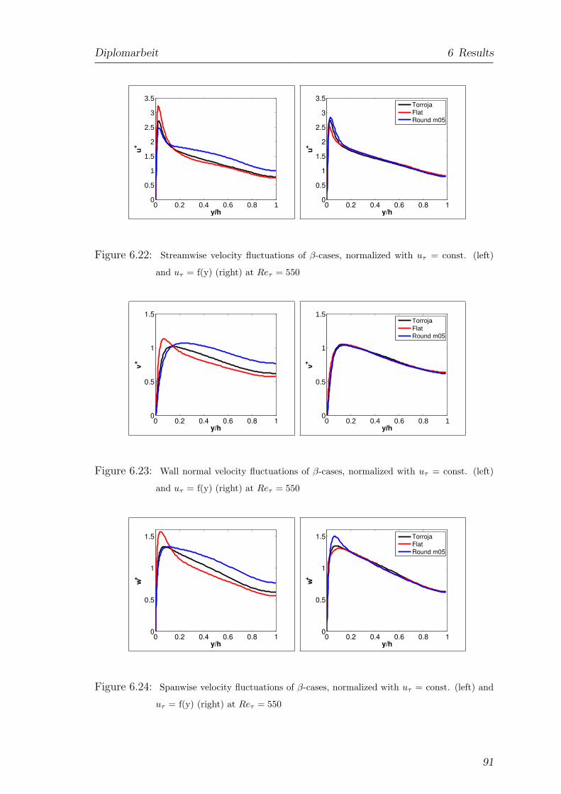
Diplomarbeit 6 Results
0 0.2 0.4 0.6 0.8 10
0.5
1
1.5
2
2.5
3
3.5
u+
y/h0 0.2 0.4 0.6 0.8 1
0
0.5
1
1.5
2
2.5
3
3.5
u+
y/h
Torroja
Flat
Round m05
Figure 6.22: Streamwise velocity fluctuations of β-cases, normalized with uτ = const. (left)
and uτ = f(y) (right) at Reτ = 550
0 0.2 0.4 0.6 0.8 10
0.5
1
1.5
v+
y/h0 0.2 0.4 0.6 0.8 1
0
0.5
1
1.5v+
y/h
TorrojaFlatRound m05
Figure 6.23: Wall normal velocity fluctuations of β-cases, normalized with uτ = const. (left)
and uτ = f(y) (right) at Reτ = 550
0 0.2 0.4 0.6 0.8 10
0.5
1
1.5
w+
y/h0 0.2 0.4 0.6 0.8 1
0
0.5
1
1.5
w+
y/h
Torroja
Flat
Round m05
Figure 6.24: Spanwise velocity fluctuations of β-cases, normalized with uτ = const. (left) and
uτ = f(y) (right) at Reτ = 550
91
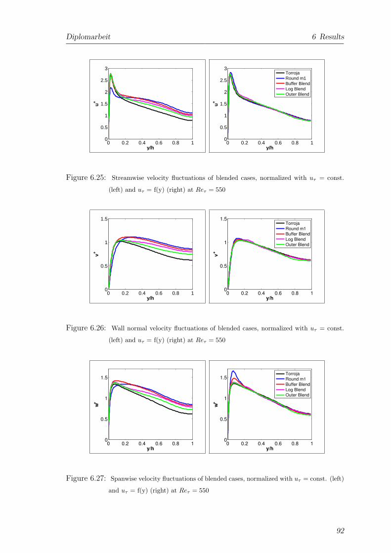
Diplomarbeit 6 Results
0 0.2 0.4 0.6 0.8 10
0.5
1
1.5
2
2.5
3
u+
y/h0 0.2 0.4 0.6 0.8 1
0
0.5
1
1.5
2
2.5
3
u+
y/h
TorrojaRound m1Buffer BlendLog BlendOuter Blend
Figure 6.25: Streamwise velocity fluctuations of blended cases, normalized with uτ = const.
(left) and uτ = f(y) (right) at Reτ = 550
0 0.2 0.4 0.6 0.8 10
0.5
1
1.5
v+
y/h0 0.2 0.4 0.6 0.8 1
0
0.5
1
1.5v+
y/h
Torroja
Round m1Buffer BlendLog BlendOuter Blend
Figure 6.26: Wall normal velocity fluctuations of blended cases, normalized with uτ = const.
(left) and uτ = f(y) (right) at Reτ = 550
0 0.2 0.4 0.6 0.8 10
0.5
1
1.5
w+
y/h0 0.2 0.4 0.6 0.8 1
0
0.5
1
1.5
w+
y/h
Torroja
Round m1Buffer BlendLog BlendOuter Blend
Figure 6.27: Spanwise velocity fluctuations of blended cases, normalized with uτ = const. (left)
and uτ = f(y) (right) at Reτ = 550
92
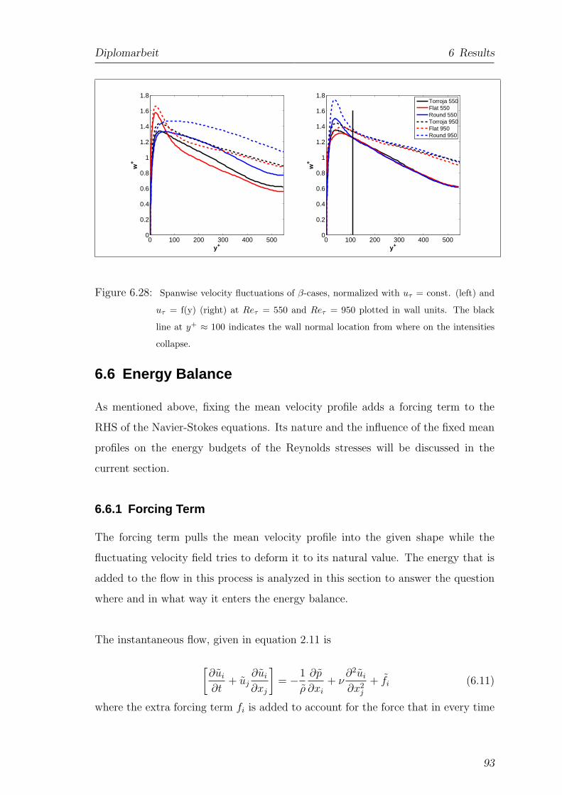
Diplomarbeit 6 Results
0 100 200 300 400 5000
0.2
0.4
0.6
0.8
1
1.2
1.4
1.6
1.8
w+
y+0 100 200 300 400 500
0
0.2
0.4
0.6
0.8
1
1.2
1.4
1.6
1.8
w+
y+
Torroja 550Flat 550Round 550Torroja 950Flat 950Round 950
Figure 6.28: Spanwise velocity fluctuations of β-cases, normalized with uτ = const. (left) and
uτ = f(y) (right) at Reτ = 550 and Reτ = 950 plotted in wall units. The black
line at y+ ≈ 100 indicates the wall normal location from where on the intensities
collapse.
6.6 Energy Balance
As mentioned above, fixing the mean velocity profile adds a forcing term to the
RHS of the Navier-Stokes equations. Its nature and the influence of the fixed mean
profiles on the energy budgets of the Reynolds stresses will be discussed in the
current section.
6.6.1 Forcing Term
The forcing term pulls the mean velocity profile into the given shape while the
fluctuating velocity field tries to deform it to its natural value. The energy that is
added to the flow in this process is analyzed in this section to answer the question
where and in what way it enters the energy balance.
The instantaneous flow, given in equation 2.11 is
[
∂ui
∂t+ uj
∂ui
∂xj
]
= −1
ρ
∂p
∂xi
+ ν∂2ui
∂x2j
+ fi (6.11)
where the extra forcing term fi is added to account for the force that in every time
93
Diplomarbeit 6 Results
step pulls the mean velocity profile back into its given place when it wants to adjust
to its natural value. The Reynolds decomposition for the velocity field and the
forcing term respectively is given by
ui = Ui + ui
fi = Fi + fi (6.12)
To the equation for the averaged velocity, which is computed by applying 6.12 on
6.11 and averaging it, the mean forcing term Fi is added. This yields
DUi
Dt= − ∂p
∂xj
+ ν∇2Ui −∂uiuj
∂xj
+ Fi (6.13)
The equation for the instantaneous fluctuating velocity is obtained by subtracting
6.11 from 6.13
[
∂ui
∂t+ Uj
∂ui
∂xj
]
= − ∂p
∂xi
+ ν∂2ui
∂x2j
−[
uj∂Ui
∂xj
]
−{
uj∂ui
∂xj
−⟨
uj∂ui
∂xj
⟩}
+ fi (6.14)
To quantify the forcing term, equations 6.13 and 6.14 are considered in Fourier
space. As mentioned before, the zero mode of the Fourier notation represent the
mean velocity profile, while the fluctuations are represented in the higher modes.
The forcing term in streamwise direction pulls the zero mode of the instnataneous
streamwise velocity component to the given value. The forcing term in spanwise
direction pulls the instantaneous value of the zero mode of the spanwise velocity
component to zero. The wall normal mean velocity profile is zero for mass conser-
vation. Therefore the forcing term f is a function of the wall normal distance y and
has entries only in the zero modes for u = U and w = W = 0 but no fluctuating
terms f = 0. If now the stress tensor⟨
f u⟩
is calculated by applying the Reynolds
decomposition from equation 6.12. This yields
⟨
fiuk
⟩
= 〈(F + f) (U + u)〉
= 〈FU + fU + Fu + fu〉 (6.15)
= 〈FU〉 (6.16)
94
Diplomarbeit 6 Results
Herefrom it becomes clear that only the term 〈FU〉 prevails, since the zero modes of
the fluctuating forcing term f are zero as well as the zero modes of the fluctuating
velocity u are zero. The resulting term F goes into the equation for the averaged
velocity given in 6.13.
The resulting tensor
〈FU〉 =
⟨
FxU FxV FxW
FyU FyV FyW
FzU FzV FzW
⟩
(6.17)
reduces to a vector
〈FU〉 =
⟨
FxU
0
0
⟩
(6.18)
since Fy = 0, V = 0 and W = 0. To see where the extra energy is fed into the
fluctuations equation 6.14 is considered.
Since the forcing term fi drops out, the only way the extra energy from the force can
enter into the fluctuations is through the mean velocity gradient in the production
term[
uj∂Ui
∂xj
]
.
To quantify the energy that is produced by the various profiles the Reynolds stress
equation is considered. In order to obtain the equation for the kinetic energy
equation, the equation for the fluctuating velocity 6.14 is multiplied by uk and
averaged. It follows
[⟨
uk∂ui
∂t
⟩
+ Uj
⟨
uk∂ui
∂xj
⟩]
= −⟨
uk∂p
∂xi
⟩
+ν
⟨
uk∂2ui
∂x2j
⟩
−[
〈ukuj〉∂Ui
∂xj
]
−⟨
ukuj∂ui
∂xj
⟩
(6.19)
Since both i and k are free indices, they can be interchanged and after some
rearragement and the decomposition of the velocity deformation rate tensor (strain
rate tensor) into its symmetric part and antisymmetric part according to
95
Diplomarbeit 6 Results
∂ui
∂xj
= sij + ωij =1
2
[
∂ui
∂xj
+∂uj
∂xi
]
+1
2
[
∂ui
∂xj
− ∂uj
∂xi
]
(6.20)
as well as the fact that the double contraction of a symmetric tensor with an anti-
symmetric tensor is identically zero, yields the equation for the Reynolds stress
〈uiuj〉 to
D 〈uiuj〉Dt
= Pij + ǫij + Tij + ΠSij + Πd
ij + Vij (6.21)
following [17], where the various terms on the right hand side are referred to as
production Pij, dissipation ǫij, turbulent diffusion Tij, pressure strain ΠSij, pressure
diffusion Πdij and viscous diffusion Vij. They are given as
Pij = −〈uiuj〉∂Uj
∂xk
− 〈uiuj〉∂Ui
∂xk
(6.22)
ǫij = −2ν
⟨
∂ui
∂xk
∂uj
∂xk
⟩
(6.23)
Tij =∂ 〈uiujuk〉
∂xk
(6.24)
ΠSij =
⟨
p
(
∂ui
∂xj
+∂uj
∂xi
)⟩
(6.25)
Πdij = − ∂
∂xk
[〈pui〉 δjk + 〈puj〉 δik] (6.26)
Vij = ν∂2 〈uiuj〉
∂x2k
(6.27)
It becomes clear again, that the extra energy seen in the statistics of total stresses,
is added to the flow through the gradient of the mean profile (production term)
from where it is then moved into the other components. Thus, the extra energy can
be computed by subtracting the total stresses of each unnatural case from the total
stress of the natural case.
The Reynolds stresses of the natural case, the round (β = −0.5) and the flat
(β = +0.5) case are shown in figure 6.29 on the left. In the middle the subtraction
of the two unnatural cases from the natural cases depict the force which tries to
pull the profile to its natural value. The multiplication with the respective mean
profile of each case yields the energy added to or taken from the flow at a given wall
96
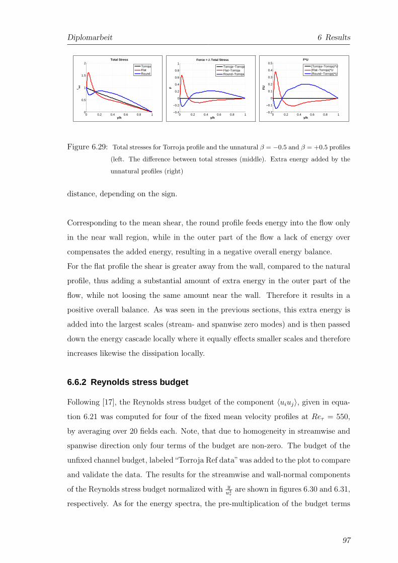
Diplomarbeit 6 Results
0 0.2 0.4 0.6 0.8 10
0.5
1
1.5
2
τ tot
y/h
Total Stress
TorrojaFlatRound
0 0.2 0.4 0.6 0.8 1−0.4
−0.2
0
0.2
0.4
0.6
0.8
1
F
y/h
Force = ∆ Total Stress
Torroja−TorrojaFlat−TorrojaRound−Torroja
0 0.2 0.4 0.6 0.8 1−0.2
−0.1
0
0.1
0.2
0.3
0.4
0.5
FU
y/h
F*U
(Torroja−Torroja)*U(Flat−Torroja)*U(Round−Torroja)*U
Figure 6.29: Total stresses for Torroja profile and the unnatural β = −0.5 and β = +0.5 profiles
(left. The difference between total stresses (middle). Extra energy added by the
unnatural profiles (right)
distance, depending on the sign.
Corresponding to the mean shear, the round profile feeds energy into the flow only
in the near wall region, while in the outer part of the flow a lack of energy over
compensates the added energy, resulting in a negative overall energy balance.
For the flat profile the shear is greater away from the wall, compared to the natural
profile, thus adding a substantial amount of extra energy in the outer part of the
flow, while not loosing the same amount near the wall. Therefore it results in a
positive overall balance. As was seen in the previous sections, this extra energy is
added into the largest scales (stream- and spanwise zero modes) and is then passed
down the energy cascade locally where it equally effects smaller scales and therefore
increases likewise the dissipation locally.
6.6.2 Reynolds stress budget
Following [17], the Reynolds stress budget of the component 〈uiuj〉, given in equa-
tion 6.21 was computed for four of the fixed mean velocity profiles at Reτ = 550,
by averaging over 20 fields each. Note, that due to homogeneity in streamwise and
spanwise direction only four terms of the budget are non-zero. The budget of the
unfixed channel budget, labeled“Torroja Ref data”was added to the plot to compare
and validate the data. The results for the streamwise and wall-normal components
of the Reynolds stress budget normalized with yu3
τare shown in figures 6.30 and 6.31,
respectively. As for the energy spectra, the pre-multiplication of the budget terms
97
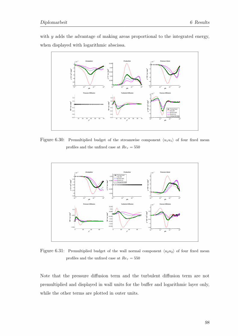
Diplomarbeit 6 Results
with y adds the advantage of making areas proportional to the integrated energy,
when displayed with logarithmic abscissa.
10−3
10−2
10−1
100
−12
−10
−8
−6
−4
−2
0
x 10−3 Dissipation
y *
D *
nu
2 / ut
au4
y/h10
−310
−210
−110
0
0
0.005
0.01
0.015
0.02
0.025
y *
P *
nu
/ uta
u4
y/h
Production
10−3
10−2
10−1
100
−10
−8
−6
−4
−2
0
x 10−3
y *
PS
* n
u / u
tau
4
y/h
Pressure Strain
10 20 30 40 50 60 70−0.4
−0.3
−0.2
−0.1
0
0.1
0.2
PD
* n
u / u
tau
4
y+
Pressure Diffusion
10 20 30 40 50 60 70−0.4
−0.3
−0.2
−0.1
0
0.1
0.2
TD
* n
u / u
tau
4
y+
Turbulent Diffusion
10−3
10−2
10−1
100
−4
−3
−2
−1
0
1
2x 10
−3
y *
VD
* n
u2 /
utau
4
y/h
Viscous Diffusion
Torroja fixedFlat p05Round m05Round m1Torroja Ref data
Figure 6.30: Premultiplied budget of the streamwise component 〈u1u1〉 of four fixed mean
profiles and the unfixed case at Reτ = 550
10−3
10−2
10−1
100
−3.5
−3
−2.5
−2
−1.5
−1
−0.5
0
x 10−3 Dissipation
y *
D *
nu
2 / ut
au4
y/h10
−310
−210
−1
−0.01
−0.005
0
0.005
0.01
y *
P *
nu
/ uta
u4
y/h
Production
10−3
10−2
10−1
100
−1
0
1
2
3
4
x 10−3
y *
PS
* n
u / u
tau
4
y/h
Pressure Strain
0 20 40 60
−0.05
0
0.05
0.1
PD
* n
u / u
tau
4
y+
Pressure Diffusion
0 20 40 60
−0.025
−0.02
−0.015
−0.01
−0.005
0
0.005
0.01
0.015
TD
* n
u / u
tau
4
y+
Turbulent Diffusion
10−3
10−2
10−1
100
−1.5
−1
−0.5
0
0.5
1
x 10−4
y *
VD
* n
u2 /
utau
4
y/h
Viscous Diffusion
Torroja fixedFlat p05Round m05Round m1Torroja Ref data
Figure 6.31: Premultiplied budget of the wall normal component 〈u2u2〉 of four fixed mean
profiles and the unfixed case at Reτ = 550
Note that the pressure diffusion term and the turbulent diffusion term are not
premultiplied and displayed in wall units for the buffer and logarithmic layer only,
while the other terms are plotted in outer units.
98
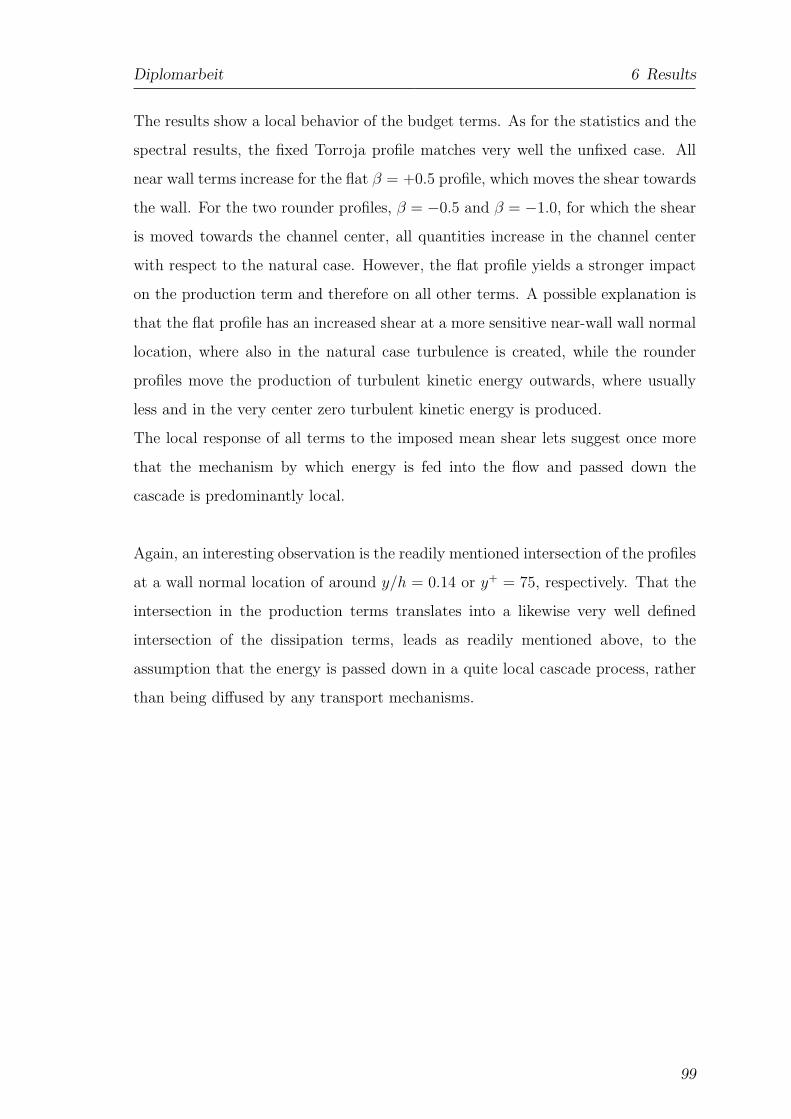
Diplomarbeit 6 Results
The results show a local behavior of the budget terms. As for the statistics and the
spectral results, the fixed Torroja profile matches very well the unfixed case. All
near wall terms increase for the flat β = +0.5 profile, which moves the shear towards
the wall. For the two rounder profiles, β = −0.5 and β = −1.0, for which the shear
is moved towards the channel center, all quantities increase in the channel center
with respect to the natural case. However, the flat profile yields a stronger impact
on the production term and therefore on all other terms. A possible explanation is
that the flat profile has an increased shear at a more sensitive near-wall wall normal
location, where also in the natural case turbulence is created, while the rounder
profiles move the production of turbulent kinetic energy outwards, where usually
less and in the very center zero turbulent kinetic energy is produced.
The local response of all terms to the imposed mean shear lets suggest once more
that the mechanism by which energy is fed into the flow and passed down the
cascade is predominantly local.
Again, an interesting observation is the readily mentioned intersection of the profiles
at a wall normal location of around y/h = 0.14 or y+ = 75, respectively. That the
intersection in the production terms translates into a likewise very well defined
intersection of the dissipation terms, leads as readily mentioned above, to the
assumption that the energy is passed down in a quite local cascade process, rather
than being diffused by any transport mechanisms.
99
Diplomarbeit 6 Results
6.7 Linear stability analysis
Even though the mean velocity profile of a channel flow is linear stable, as can be
seen in figure 6.32, since the imaginary parts of all eigenvalues are negative, linear
perturbations can grow substantially before they decay by extracting energy from
the mean flow. This transient energy amplifications was linked by [8] to coherent
structures in wall-bounded turbulence.
For an instable profile only one eigenvalue has to become positive. Transient growth
however is the result of the combination of multiple stable eigenvalues, which for the
current streamwise and spanwise perturbation wave numbers α ≈ 1.75, β ≈ 0.30 is
depicted in the light green box in figure 6.32.
Two peaks of the transient growth were found in natural channel flows by [8].
One in the viscous layer and one in the outer layer. The peak in the viscous
layer identifies the sublayer streaks while in the outer layer it identifies the large
scale global structures, that span the full channel. The minimum in between the
two most amplified modes corresponds to the structures in the log-layer. In the
present work linear analysis of the most amplified transient modes was used to
obtain further insight into the dynamics of the nonphysical turbulent flow with a
fixed mean velocity profile.
In general it is assumed that the small structures in the viscous layer equilibrate
with their large-scale environment. By fixing the mean profile, and especially by
fixing it to wrong values it was tried to gain further insights into those mechanisms.
Also, the cycle mechanisms, that are involved in the deformation of the mean profile,
are of interest to the present work, since it would be disrupted or at least falsified,
by fixing the mean profile to the correct or to a wrong profile, respectively. Thus,
by using the linear stability analysis it is expected to gather further insight into
what kind of structures are created by the various profiles and how the interaction
mechanisms work.
The procedure will be shortly explained in the following section before the results
100
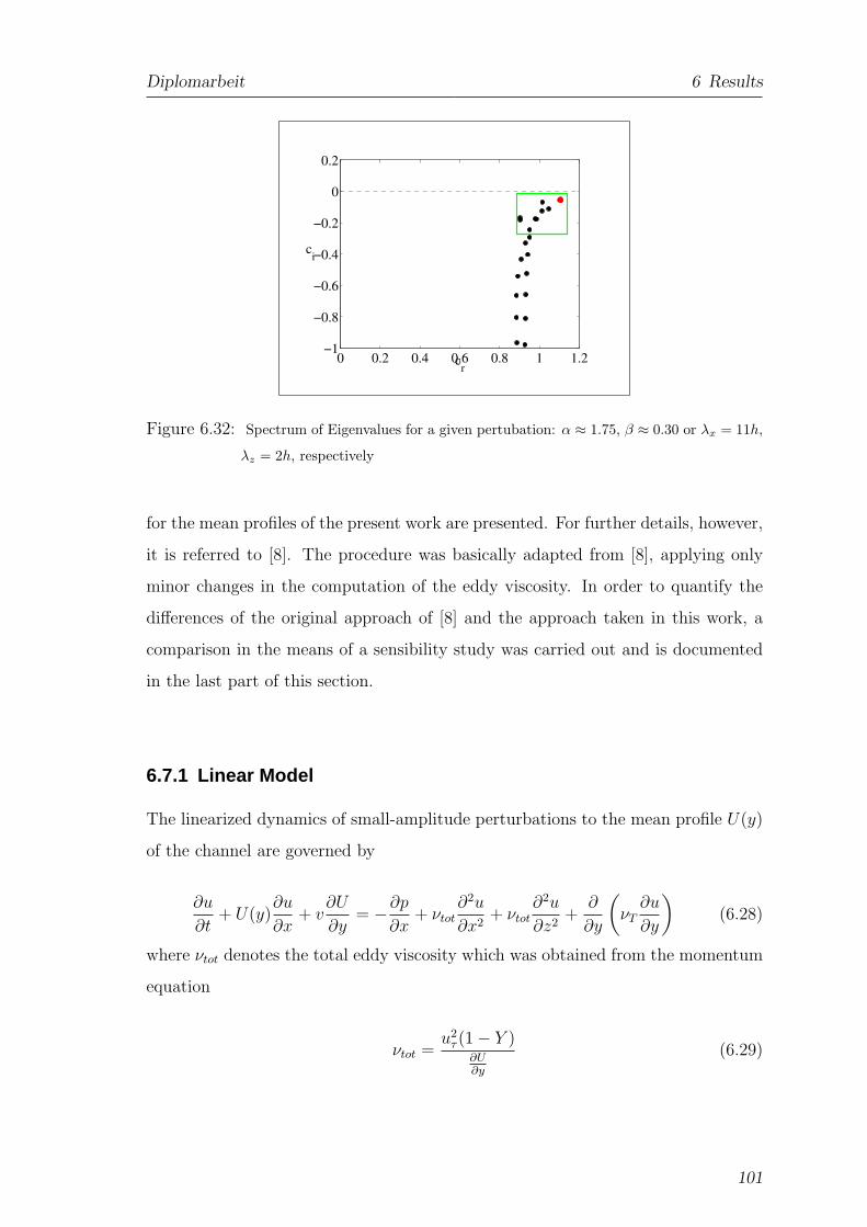
Diplomarbeit 6 Results
0 0.2 0.4 0.6 0.8 1 1.2−1
−0.8
−0.6
−0.4
−0.2
0
0.2
cr
ci
Figure 6.32: Spectrum of Eigenvalues for a given pertubation: α ≈ 1.75, β ≈ 0.30 or λx = 11h,
λz = 2h, respectively
for the mean profiles of the present work are presented. For further details, however,
it is referred to [8]. The procedure was basically adapted from [8], applying only
minor changes in the computation of the eddy viscosity. In order to quantify the
differences of the original approach of [8] and the approach taken in this work, a
comparison in the means of a sensibility study was carried out and is documented
in the last part of this section.
6.7.1 Linear Model
The linearized dynamics of small-amplitude perturbations to the mean profile U(y)
of the channel are governed by
∂u
∂t+ U(y)
∂u
∂x+ v
∂U
∂y= −∂p
∂x+ νtot
∂2u
∂x2+ νtot
∂2u
∂z2+
∂
∂y
(
νT∂u
∂y
)
(6.28)
where νtot denotes the total eddy viscosity which was obtained from the momentum
equation
νtot =u2
τ (1 − Y )∂U∂y
(6.29)
101
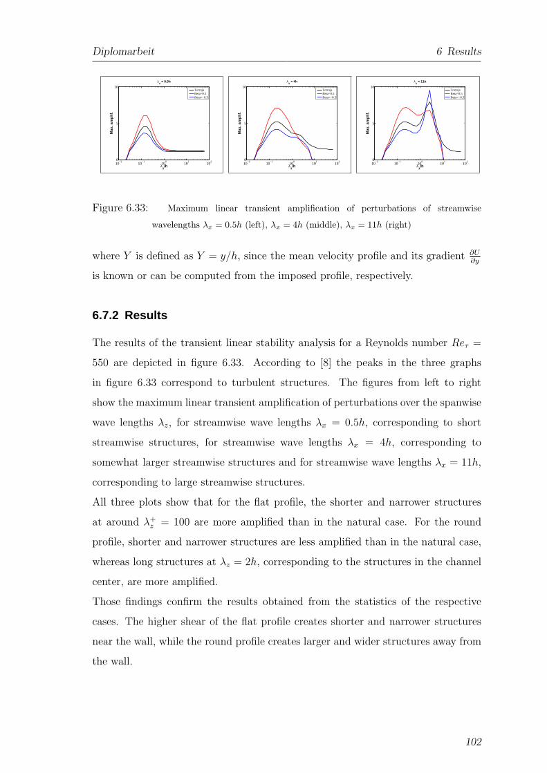
Diplomarbeit 6 Results
10−2
10−1
100
101
1020
5
10
λz/h
Max
. am
plif.
λx = 0.5h
TorrojaBeta=0.5Beta=−0.5
10−2
10−1
100
101
1020
5
10
λz/h
Max
. am
plif.
λx = 4h
TorrojaBeta=0.5Beta=−0.5
10−2
10−1
100
101
1020
5
10
λz/h
Max
. am
plif.
λx = 11h
TorrojaBeta=0.5Beta=−0.5
Figure 6.33: Maximum linear transient amplification of perturbations of streamwise
wavelengths λx = 0.5h (left), λx = 4h (middle), λx = 11h (right)
where Y is defined as Y = y/h, since the mean velocity profile and its gradient ∂U∂y
is known or can be computed from the imposed profile, respectively.
6.7.2 Results
The results of the transient linear stability analysis for a Reynolds number Reτ =
550 are depicted in figure 6.33. According to [8] the peaks in the three graphs
in figure 6.33 correspond to turbulent structures. The figures from left to right
show the maximum linear transient amplification of perturbations over the spanwise
wave lengths λz, for streamwise wave lengths λx = 0.5h, corresponding to short
streamwise structures, for streamwise wave lengths λx = 4h, corresponding to
somewhat larger streamwise structures and for streamwise wave lengths λx = 11h,
corresponding to large streamwise structures.
All three plots show that for the flat profile, the shorter and narrower structures
at around λ+z = 100 are more amplified than in the natural case. For the round
profile, shorter and narrower structures are less amplified than in the natural case,
whereas long structures at λz = 2h, corresponding to the structures in the channel
center, are more amplified.
Those findings confirm the results obtained from the statistics of the respective
cases. The higher shear of the flat profile creates shorter and narrower structures
near the wall, while the round profile creates larger and wider structures away from
the wall.
102
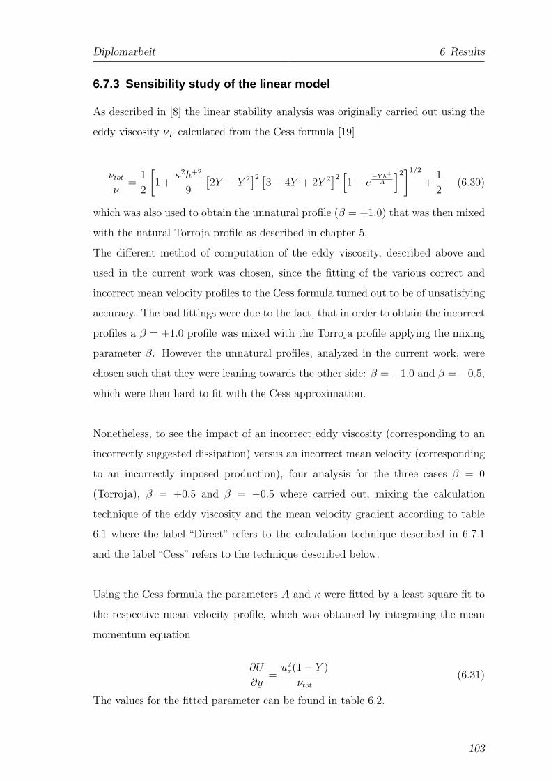
Diplomarbeit 6 Results
6.7.3 Sensibility study of the linear model
As described in [8] the linear stability analysis was originally carried out using the
eddy viscosity νT calculated from the Cess formula [19]
νtot
ν=
1
2
[
1 +κ2h+2
9
[
2Y − Y 2]2 [
3 − 4Y + 2Y 2]2
[
1 − e−Y h+
A
]2]1/2
+1
2(6.30)
which was also used to obtain the unnatural profile (β = +1.0) that was then mixed
with the natural Torroja profile as described in chapter 5.
The different method of computation of the eddy viscosity, described above and
used in the current work was chosen, since the fitting of the various correct and
incorrect mean velocity profiles to the Cess formula turned out to be of unsatisfying
accuracy. The bad fittings were due to the fact, that in order to obtain the incorrect
profiles a β = +1.0 profile was mixed with the Torroja profile applying the mixing
parameter β. However the unnatural profiles, analyzed in the current work, were
chosen such that they were leaning towards the other side: β = −1.0 and β = −0.5,
which were then hard to fit with the Cess approximation.
Nonetheless, to see the impact of an incorrect eddy viscosity (corresponding to an
incorrectly suggested dissipation) versus an incorrect mean velocity (corresponding
to an incorrectly imposed production), four analysis for the three cases β = 0
(Torroja), β = +0.5 and β = −0.5 where carried out, mixing the calculation
technique of the eddy viscosity and the mean velocity gradient according to table
6.1 where the label “Direct” refers to the calculation technique described in 6.7.1
and the label “Cess” refers to the technique described below.
Using the Cess formula the parameters A and κ were fitted by a least square fit to
the respective mean velocity profile, which was obtained by integrating the mean
momentum equation
∂U
∂y=
u2τ (1 − Y )
νtot
(6.31)
The values for the fitted parameter can be found in table 6.2.
103
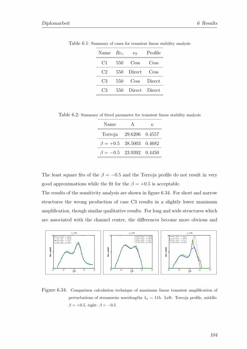
Diplomarbeit 6 Results
Table 6.1: Summary of cases for transient linear stability analysis
Name Reτ νT Profile
C1 550 Cess Cess
C2 550 Direct Cess
C3 550 Cess Direct
C3 550 Direct Direct
Table 6.2: Summary of fitted parameter for transient linear stability analysis
Name A κ
Torroja 29.6206 0.4557
β = +0.5 38.5003 0.4682
β = −0.5 23.9392 0.4450
The least square fits of the β = −0.5 and the Torroja profile do not result in very
good approximations while the fit for the β = +0.5 is acceptable.
The results of the sensitivity analysis are shown in figure 6.34. For short and narrow
structures the wrong production of case C3 results in a slightly lower maximum
amplification, though similar qualitative results. For long and wide structures which
are associated with the channel center, the differences become more obvious and
10−2
10−1
100
101
1020
5
10
λz/h
Max
. am
plif.
λx = 11h
nut = direct, u = directnut = Cess, u = directnut = direct, u = Cessnut = Cess, u = Cess
10−2
10−1
100
101
1020
5
10
λz/h
Max
. am
plif.
λx = 11h
nut = direct, u = directnut = Cess, u = directnut = direct, u = Cessnut = Cess, u = Cess
10−2
10−1
100
101
1020
5
10
λz/h
Max
. am
plif.
λx = 11h
nut = direct, u = directnut = Cess, u = directnut = direct, u = Cessnut = Cess, u = Cess
Figure 6.34: Comparison calculation technique of maximum linear transient amplification of
perturbations of streamwise wavelengths λx = 11h. Left: Torroja profile, middle:
β = +0.5, right: β = −0.5
104
Diplomarbeit 6 Results
especially so for the round (β = −0.5) profile which makes sense since the worst fit
was obtained for this profile.
By taking a closer look at the results of the (β = −0.5) profile, it can be seen that an
incorrect dissipation (dashed red line) predicts a stronger maximum amplification for
large structures in the channel center only. However, when an incorrect production
(dotted blue line) is used, the maximum amplification drops for the small near wall
structures as well as for the large structures associated with the channel center.
Interestingly the two effect cancel out each other to a certain extend and when
both, the incorrect production and the incorrect dissipation are used, the maximum
amplification (dashed green line) is somewhat closer to the correct case (solid black
line).
It can be summarized, that maximum amplification is sensitive to the calculation
technique and a bad fit of the Cess parameters can lead to erroneous results.
However, the qualitative features could be reproduced by using even badly fitted
mean profiles.
105
Diplomarbeit 6 Results
6.8 Coherent Structures
In this section the influence of a fixed mean velocity profile on the formation
of coherent structures, namely clusters, is studied. The identification method of
vortices, which form a particular kind of coherent structures, is briefly outlined,
following the results of the analysis.
To identify coherent structures in turbulent flows, the model proposed in [13], based
on [14], was used in the current work. According to [14], a coherent structure
is defined as a region in space where the velocity gradient tensor A = ∇u is
dominated by its rotational part. Using this definition and expressing it in terms
of the discriminant D the velocity gradient tensor, expressed in terms of the tensor
invariants of A, R and Q
D =27
4R2 + Q3, (6.32)
the condition translates into D > 0. To visualize the structure, a point x is
considered being a part of a vortex cluster if
D(x) > α
√
D′2(y) (6.33)
where α is the threshold parameter which can be chosen to visualize vortices of
different intensities and
√
D′2(y) is the standard deviation of D in planes parallel
to the wall. The value used in the present work to identify the vortices individually
is α = 0.02, as proposed and reasoned by [13]. The advantage of using
√
D′2(y)
instead of D(x) > α is, that the inhomogeneity from the wall can be reduced. If
D(x) > α was used, and α was set to depict coherent structures near the wall, the
channel center would appear empty. For each case the respective standard deviation
was computed individually, since D varies with the sixth order of the mean shear(
dUdy
)6
. Figure 6.35 shows the standard deviation over the wall normal distance y/h
for the all four cases analyzed. The data was obtained by averaging over 20 flow
fields. As expected, the standard deviation changes accordingly to the mean shear.
Figure 6.36 shows the coherent structures of instantaneous flow fields in the con-
106
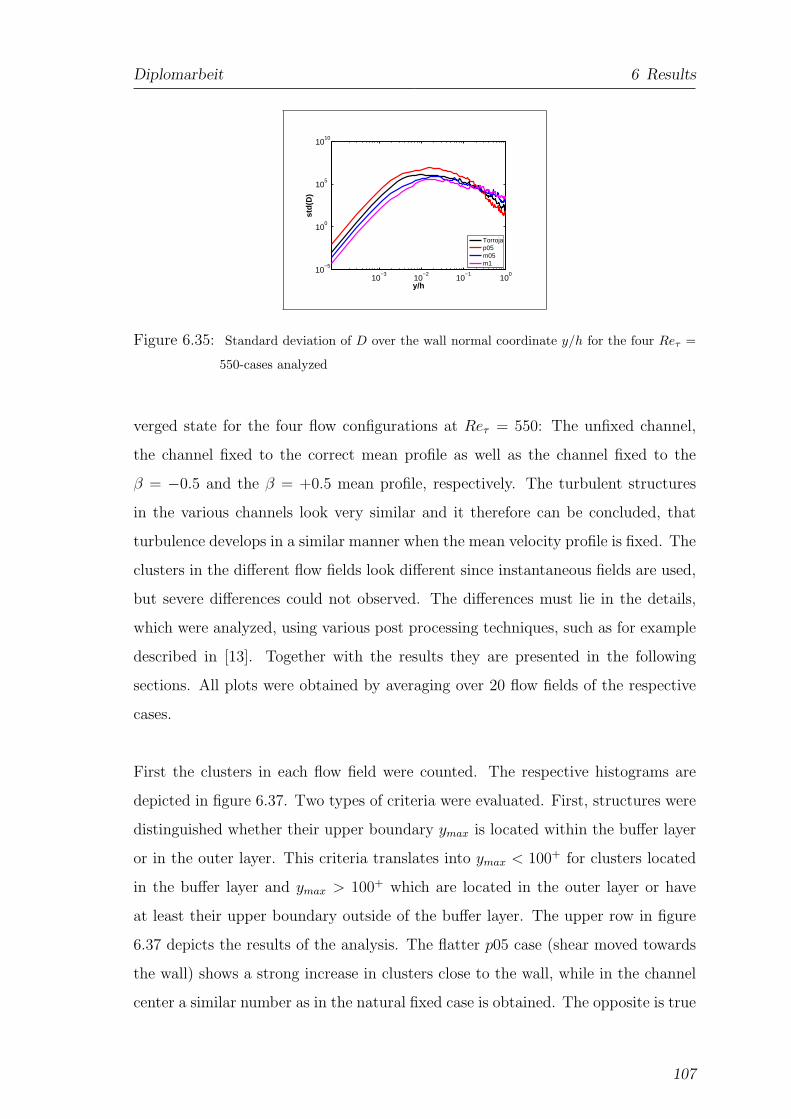
Diplomarbeit 6 Results
10−3
10−2
10−1
100
10−5
100
105
1010
std(
D)
y/h
Torrojap05m05m1
Figure 6.35: Standard deviation of D over the wall normal coordinate y/h for the four Reτ =
550-cases analyzed
verged state for the four flow configurations at Reτ = 550: The unfixed channel,
the channel fixed to the correct mean profile as well as the channel fixed to the
β = −0.5 and the β = +0.5 mean profile, respectively. The turbulent structures
in the various channels look very similar and it therefore can be concluded, that
turbulence develops in a similar manner when the mean velocity profile is fixed. The
clusters in the different flow fields look different since instantaneous fields are used,
but severe differences could not observed. The differences must lie in the details,
which were analyzed, using various post processing techniques, such as for example
described in [13]. Together with the results they are presented in the following
sections. All plots were obtained by averaging over 20 flow fields of the respective
cases.
First the clusters in each flow field were counted. The respective histograms are
depicted in figure 6.37. Two types of criteria were evaluated. First, structures were
distinguished whether their upper boundary ymax is located within the buffer layer
or in the outer layer. This criteria translates into ymax < 100+ for clusters located
in the buffer layer and ymax > 100+ which are located in the outer layer or have
at least their upper boundary outside of the buffer layer. The upper row in figure
6.37 depicts the results of the analysis. The flatter p05 case (shear moved towards
the wall) shows a strong increase in clusters close to the wall, while in the channel
center a similar number as in the natural fixed case is obtained. The opposite is true
107
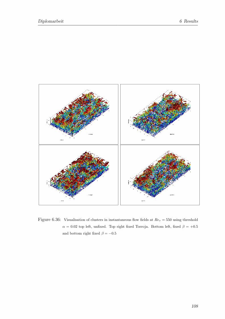
Diplomarbeit 6 Results
Figure 6.36: Visualisation of clusters in instantaneous flow fields at Reτ = 550 using threshold
α = 0.02 top left, unfixed. Top right fixed Torroja. Bottom left, fixed β = +0.5
and bottom right fixed β = −0.5
108
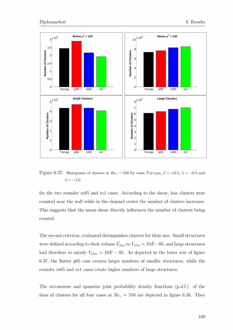
Diplomarbeit 6 Results
Torroja p05 m05 m10
0.5
1
1.5
2
2.5
3x 10
4
Num
ber
of C
lust
ers
Below y + = 100
Torroja p05 m05 m10
2
4
6
8
10x 10
4
Num
ber
of C
lust
ers
Above y + = 100
Torroja p05 m05 m10
1
2
3
4
5x 10
4
Num
ber
of C
lust
ers
Small Clusters
Torroja p05 m05 m10
1
2
3
4
5
6
7
8x 10
4
Num
ber
of C
lust
ers
Large Clusters
Figure 6.37: Histograms of clusters at Reτ = 550 for cases Torroja, β = +0.5, β = −0.5 and
β = −1.0
for the two rounder m05 and m1 cases. According to the shear, less clusters were
counted near the wall while in the channel center the number of clusters increases.
This suggests that the mean shear directly influences the number of clusters being
created.
The second criterion, evaluated distinguishes clusters for their size. Small structures
were defined according to their volume Vclus to Vclus < 10E−05, and large structures
had therefore to satisfy Vclus > 10E − 05. As depicted in the lower row of figure
6.37, the flatter p05 case creates larger numbers of smaller structures, while the
rounder m05 and m1 cases create higher numbers of large structures.
The streamwise and spanwise joint probability density functions (p.d.f.) of the
sizes of clusters for all four cases at Reτ = 550 are depicted in figure 6.38. They
109
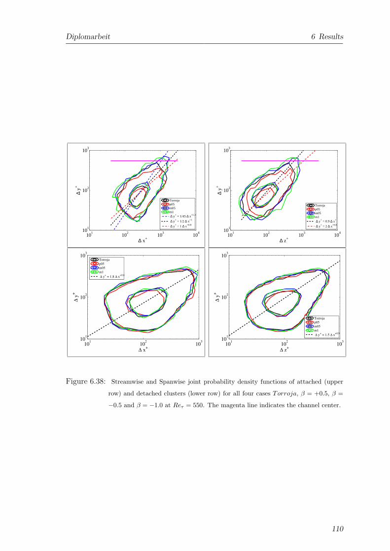
Diplomarbeit 6 Results
101
102
103
10410
1
102
103
∆ x+
∆ y+
Torrojap05m05m1 ∆ y+ = 1/45 ∆ x+1.3
∆ y+ = 1/2 ∆ x+1
∆ y+ = 1 ∆ x+0.8
101
102
103
10410
1
102
103
∆ z+
∆ y+
Torrojap05m05m1 ∆ y+ = 0.9 ∆ x+
∆ y+ = 2 ∆ x+0.8
101
102
103
101
102
103
∆ x+
∆y+
Torroja
p05
m05
m1
∆ y+= 1.8 ∆ x
+0.8
101
102
103
101
102
103
∆ z+
∆y+
Torroja
p05
m05
m1
∆ y+= 1.5 ∆ x
+0.9
Figure 6.38: Streamwise and Spanwise joint probability density functions of attached (upper
row) and detached clusters (lower row) for all four cases Torroja, β = +0.5, β =
−0.5 and β = −1.0 at Reτ = 550. The magenta line indicates the channel center.
110
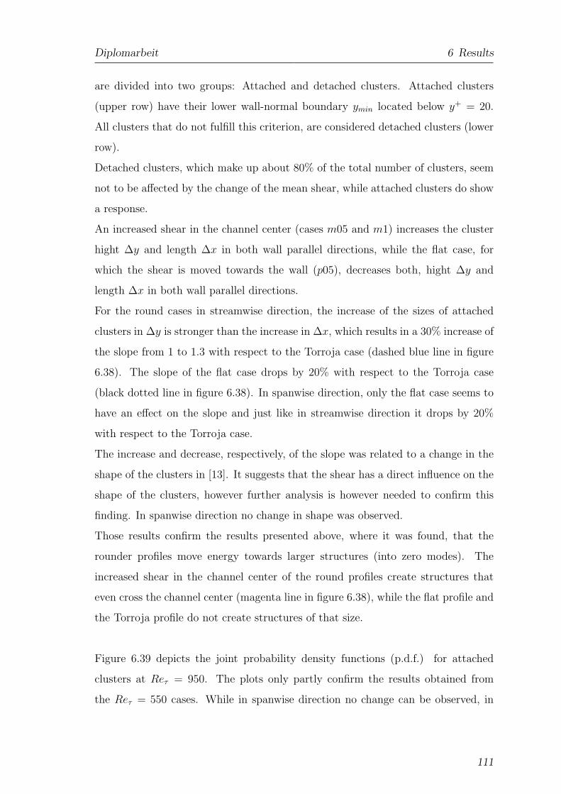
Diplomarbeit 6 Results
are divided into two groups: Attached and detached clusters. Attached clusters
(upper row) have their lower wall-normal boundary ymin located below y+ = 20.
All clusters that do not fulfill this criterion, are considered detached clusters (lower
row).
Detached clusters, which make up about 80% of the total number of clusters, seem
not to be affected by the change of the mean shear, while attached clusters do show
a response.
An increased shear in the channel center (cases m05 and m1) increases the cluster
hight ∆y and length ∆x in both wall parallel directions, while the flat case, for
which the shear is moved towards the wall (p05), decreases both, hight ∆y and
length ∆x in both wall parallel directions.
For the round cases in streamwise direction, the increase of the sizes of attached
clusters in ∆y is stronger than the increase in ∆x, which results in a 30% increase of
the slope from 1 to 1.3 with respect to the Torroja case (dashed blue line in figure
6.38). The slope of the flat case drops by 20% with respect to the Torroja case
(black dotted line in figure 6.38). In spanwise direction, only the flat case seems to
have an effect on the slope and just like in streamwise direction it drops by 20%
with respect to the Torroja case.
The increase and decrease, respectively, of the slope was related to a change in the
shape of the clusters in [13]. It suggests that the shear has a direct influence on the
shape of the clusters, however further analysis is however needed to confirm this
finding. In spanwise direction no change in shape was observed.
Those results confirm the results presented above, where it was found, that the
rounder profiles move energy towards larger structures (into zero modes). The
increased shear in the channel center of the round profiles create structures that
even cross the channel center (magenta line in figure 6.38), while the flat profile and
the Torroja profile do not create structures of that size.
Figure 6.39 depicts the joint probability density functions (p.d.f.) for attached
clusters at Reτ = 950. The plots only partly confirm the results obtained from
the Reτ = 550 cases. While in spanwise direction no change can be observed, in
111
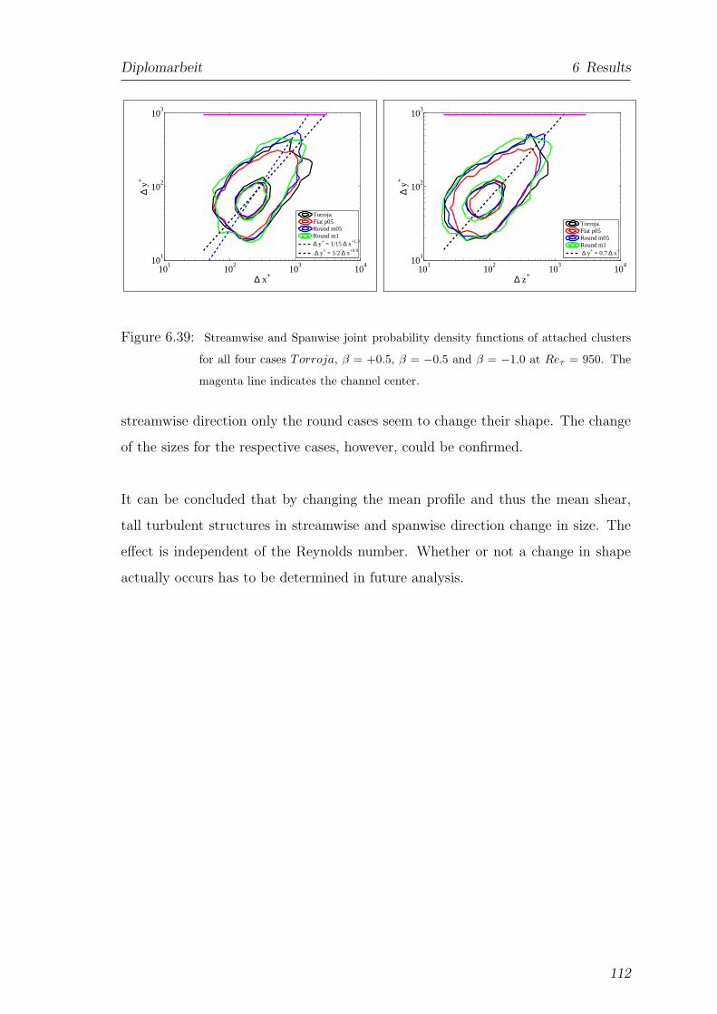
Diplomarbeit 6 Results
101
102
103
10410
1
102
103
∆ x+
∆ y+
TorrojaFlat p05Round m05Round m1∆ y+ = 1/15 ∆ x+1.3
∆ y+ = 1/2 ∆ x+0.9
101
102
103
10410
1
102
103
∆ z+
∆ y+
TorrojaFlat p05Round m05Round m1 ∆ y+ = 0.7 ∆ x+
Figure 6.39: Streamwise and Spanwise joint probability density functions of attached clusters
for all four cases Torroja, β = +0.5, β = −0.5 and β = −1.0 at Reτ = 950. The
magenta line indicates the channel center.
streamwise direction only the round cases seem to change their shape. The change
of the sizes for the respective cases, however, could be confirmed.
It can be concluded that by changing the mean profile and thus the mean shear,
tall turbulent structures in streamwise and spanwise direction change in size. The
effect is independent of the Reynolds number. Whether or not a change in shape
actually occurs has to be determined in future analysis.
112
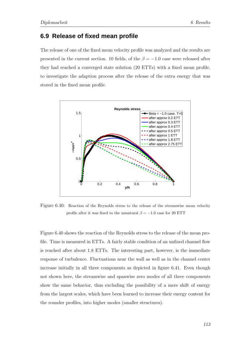
Diplomarbeit 6 Results
6.9 Release of fixed mean profile
The release of one of the fixed mean velocity profile was analyzed and the results are
presented in the current section. 10 fields, of the β = −1.0 case were released after
they had reached a converged state solution (20 ETTs) with a fixed mean profile,
to investigate the adaption process after the release of the extra energy that was
stored in the fixed mean profile.
0 0.2 0.4 0.6 0.8 10
0.5
1
1.5
−<uv
>+
y/h
Reynolds stress
Beta = −1.0 case. T=0after approx 0.2 ETTafter approx 0.3 ETTafter approx 0.4 ETTafter approx 0.5 ETTafter approx 1 ETTafter approx 1.8 ETTafter approx 2.75 ETT
Figure 6.40: Reaction of the Reynolds stress to the release of the streamwise mean velocity
profile after it was fixed to the unnatural β = −1.0 case for 20 ETT
Figure 6.40 shows the reaction of the Reynolds stress to the release of the mean pro-
file. Time is measured in ETTs. A fairly stable condition of an unfixed channel flow
is reached after about 1.8 ETTs. The interesting part, however, is the immediate
response of turbulence. Fluctuations near the wall as well as in the channel center
increase initially in all three components as depicted in figure 6.41. Even though
not shown here, the streamwise and spanwise zero modes of all three components
show the same behavior, thus excluding the possibility of a mere shift of energy
from the largest scales, which have been learned to increase their energy content for
the rounder profiles, into higher modes (smaller structures).
113
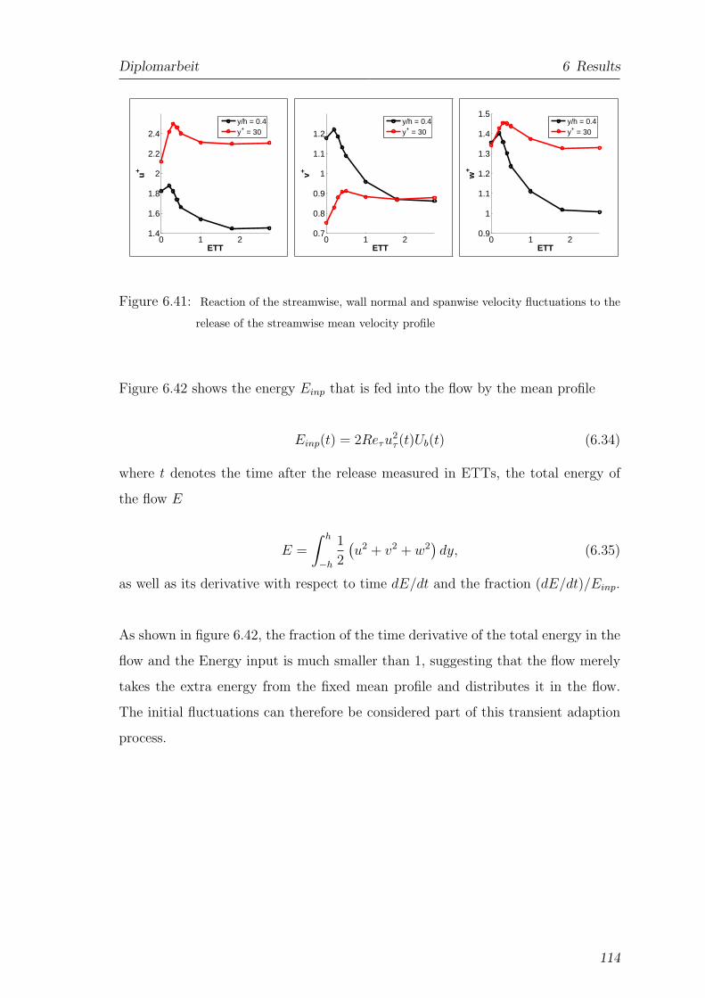
Diplomarbeit 6 Results
0 1 21.4
1.6
1.8
2
2.2
2.4u
+
ETT
y/h = 0.4y+ = 30
0 1 20.7
0.8
0.9
1
1.1
1.2
v+
ETT
y/h = 0.4y+ = 30
0 1 20.9
1
1.1
1.2
1.3
1.4
1.5
w+
ETT
y/h = 0.4y+ = 30
Figure 6.41: Reaction of the streamwise, wall normal and spanwise velocity fluctuations to the
release of the streamwise mean velocity profile
Figure 6.42 shows the energy Einp that is fed into the flow by the mean profile
Einp(t) = 2Reτu2τ (t)Ub(t) (6.34)
where t denotes the time after the release measured in ETTs, the total energy of
the flow E
E =
∫ h
−h
1
2
(
u2 + v2 + w2)
dy, (6.35)
as well as its derivative with respect to time dE/dt and the fraction (dE/dt)/Einp.
As shown in figure 6.42, the fraction of the time derivative of the total energy in the
flow and the Energy input is much smaller than 1, suggesting that the flow merely
takes the extra energy from the fixed mean profile and distributes it in the flow.
The initial fluctuations can therefore be considered part of this transient adaption
process.
114
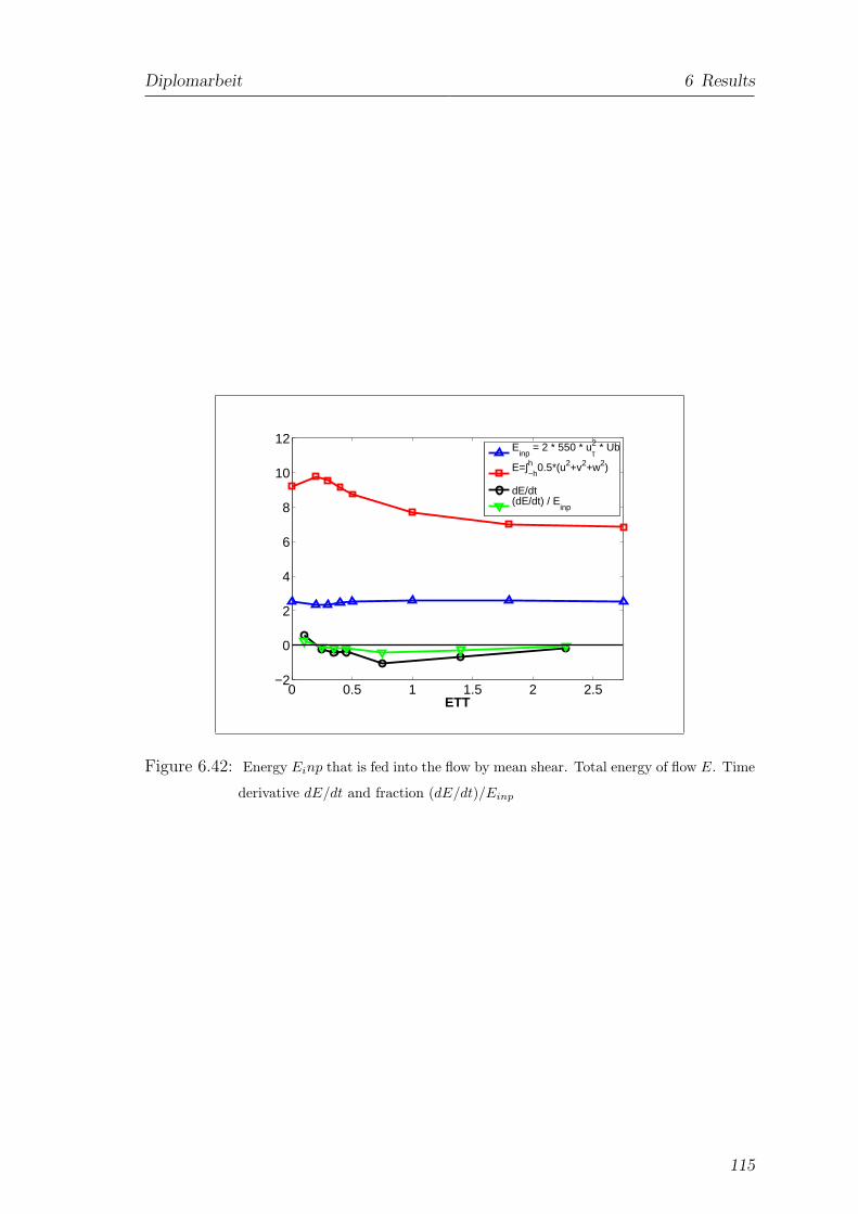
Diplomarbeit 6 Results
0 0.5 1 1.5 2 2.5−2
0
2
4
6
8
10
12
ETT
Einp
= 2 * 550 * uτ2 * Ub
E=∫−hh 0.5*(u2+v2+w2)
dE/dt(dE/dt) / E
inp
Figure 6.42: Energy Einp that is fed into the flow by mean shear. Total energy of flow E. Time
derivative dE/dt and fraction (dE/dt)/Einp
115
7 Discussion and Conclusions
To investigate systematically the effect of a fixed mean profile, several direct numer-
ical simulations with mean profiles fixed to various unnatural and blended cases, as
well as to the natural case, were carried out and the results of their post processing
were presented.
One of the central problems of wall-bounded turbulence is how structures of different
sizes, associated with different wall distances, adjust their relative intensities to
balance the mean momentum transfer in wall-normal direction. As mentioned in
the introduction, it is understood that Reynolds stresses and the mean velocity
gradient (mean shear) interact with each other to produce turbulence, but the way
how they do it is still not completely understood [7].
If a feedback mechanism between the Reynolds stresses and the mean shear exists,
which would suggest that locally weak structures, with weak Reynolds stresses,
result in a local acceleration of the mean velocity profile, which leads to local
enhancement of the velocity gradient and thus to the strengthening of the local
fluctuations, it would be disturbed by fixing the mean velocity profile and thus the
mean velocity gradient.
Interestingly, this feedback mechanism seems not to exist, since when the correct
profile is imposed, all statistical and spectral results are essentially identical, within
the statistical uncertainty, to the case when the profile is left unfixed and can evolve
according to its own equation of motion.
If however, only a slightly incorrect profile is imposed on the flow as a fixed mean ve-
116
Diplomarbeit 7 Discussion and Conclusions
locity profile, the fluctuations react highly sensitive. The statistical results showed,
that the increase or decrease of the intensities, respectively, coincides with the
gradient of the mean velocity profile. An increased mean velocity gradient results in
higher intensities and therefore higher production of turbulent kinetic energy, that
is, as was reasoned, the only way in which the extra energy from the changed mean
shear can enter the fluctuations. Following the production, it was shown, that the
dissipation peaks and drops quite locally, where the mean shear is changed.
Those results suggests, that the mean velocity gradient seems to determine the
energy that locally flows into fluctuations of a given size, which grow until they
activate an energy transfer, that is strong enough to balance the production. The
local production likewise balances the local dissipation, which is proportional to the
cube of the fluctuation intensities. This model is supported by the Reynolds budget
as well as by the results of the two dimensional energy spectra, which show, that for
a given wall distance not only the large scale fluctuations, but all scales, all the way
down to quantities like the vorticity, are effected in the same way, by the change in
the mean shear.
Rather than a feedback mechanism, the results suggest, that the intensities are
determined in a uni-directional causal chain, in which the mean shear determines
them locally and not by an interaction among structures at different wall distances.
An increased mean velocity gradient results in increased production of fluctuations,
which likewise results in an increase in vorticity and therefore dissipation, suggesting
that the whole cascade process takes place quite locally.
Furthermore, by using linear stability analysis of transient growth, it was shown,
that the changed mean shear could directly be related to the amplification of
structures at that given wall distance. This finding also supported the suggestion
of a local rather than interactive determination of the energy that is fed into the
fluctuations.
117
Diplomarbeit 7 Discussion and Conclusions
Further insights into the interaction of mean shear and fluctuations were gained
by blending two profiles, using the natural profile in the near wall region and an
unnatural (increase mean shear) in the channel center. The increased shear in the
channel center as well as the blending itself created large structures, that extend all
the way to the wall and induce Reynolds stresses in other parts of the channel. The
small structures of the two near wall blends adapted fast to the respective “mother
profile”supporting the locality of the mechanism by which energy is fed into the flow.
Those findings were confirmed by dividing the energy spectrum in the zero-zero
mode (mean profile), the zero modes (large scales) and the non zero modes (smaller
scales). All fixed cases with an increased shear in the channel center (round and
blended) show the tendency to increase the energy in the zero modes kx and kz of
the wall parallel planes, for the entire channel hight, while the flat case with less
shear in the channel center decreases its energy content in the large scales. This
suggest, that the large structures, that are created by the increased shear in the
channel center extent all the way to the wall and also implies that the mean profile
preferably interacts with scales of similar sizes. However, since all scales at a given
wall distance show the same reaction to a changed mean profile (fluctuations as well
as vorticity), it can be assumed that the cascade process acts locally and faster than
the time scale of the large eddies.
A new local velocity scale was introduced, using the square root of the total stress
for a given wall-normal distance, thus taking into account the local situation of the
Reynolds stresses. The fluctuations for all unnatural and natural profiles collapse
to the nominal value of the reference profile. Close to the wall, where the viscous
stress dominates, the scaling does not work for all components of the intensities.
By comparing the results of both Reynolds number cases, the threshold was found
to be y+ ≈ 100. This once more strongly suggests that the mechanism with which
energy is fed into velocity fluctuation is local, rather than an interaction between
eddies at different wall distances and once more support the assumption that the
intensities are determined locally and neither through interaction of structures at
118
Diplomarbeit 7 Discussion and Conclusions
different wall distances, nor through any kind of feedback mechanism.
The analysis of coherent structures (clusters) showed that turbulence develops at
first sight seemingly natural. The instantaneous field plots of the discriminant of
the velocity gradient tensor look very similar. A closer look however shows, that
by changing the mean shear, the size as well as possibly the shape of tall attached
clusters are affected. Detached clusters seem not to be affected by the changed
mean shear. This suggests that the mean shear only has an affect on large scales,
but leave smaller scales unaffected and therefore implies that it does predominantly
interact with structures of similar sizes.
An increased shear in the channel center favors the formation of large attached
“inactive” energy containing eddies. An increased shear close to the wall, however,
favors the formation of smaller, more isotropic and thus “active” structures that can
directly take part in the isotropic cascade process.
Realeasing the mean profile after the channel reached a converged state in the
unnatural configuration, showed that the adaption process happens within about 2
to 3 ETTs. The extra energy, released after releasing the mean profile settles to the
nominal value after initial fluctuations.
119
Bibliography
[1] POPE, Stephen B. 2000 Turbulent Flows, Cambridge University Press
[2] KIM, J. & MOIN, P.& MOSER, R.D. 1986 Turbulence statistics in fully
developed channel flow at low Reynolds number, J. Fluid Mech. (1987), vol.
177, pp. 133-166
[3] BOYD, John P. 2000 Chebyshev and Fourier Spectral Methods, Second
Edition, Dover Publications
[4] JIMENEZ, Javier. 2004 Turbulence and Vortex Dynamics
[5] DEL ALAMO, J.C. & JIMEENEZ, J. & ZANDONADE, P. & MOSER, R.D.
2004 Scaling of the energy spectra of turbulent channels, J. Fluid Mech. vol
500, pp 135-144
[6] JIMENEZ, Javier. 2007 Recent developments on wall-bounded turbulence,
RACSAM Vol. 101(2), pp. 187-203
[7] GEORGE, William, Lectures in Turbulence for the 21st Century, Department
of Applied Mechanics Chalmers University of Technology Gothenburg, Sweden
[8] DEL ALAMO, Juan-Carlos & JIMEENEZ, Javier. 2006 Linear energy
amplification in turbulent channels, J. Fluid Mech. 559, 205-213.
[9] SCHMID, P. J. & HENNINGSON, D.S. 2001 Stability and Transition in Shear
Flows. Springer Volume 142
[10] JIMEENEZ, Javier. 2011 Cascades in wall-bounded turbulence, Annu. Rev.
Fluid Mech. 2012 44
120
Diplomarbeit Bibliography
[11] HOYAS, Sergio & JIMEENEZ, Javier. 2006 Scaling of the velocity fluctuations
in turbulent cahnnels up to Reτ = 2003. Phys. Fluids 18:011702
[12] JIMEENEZ, Javier & Genta Kawahara. 2010 Dynamics of wall-bounded
turbulence
[13] DEL ALAMO, J.C. & JIMEENEZ, Javier & Zandonade,& Moser R.D. 2006
Self-similar vortex clusters in the logarithmic region. J. Fluid Mech., 561:329 -
358
[14] CHONG, M. S., PERRY & A. E. & CANTWELL, B. J. 1990 A general
classification of three-dimensional flow fields. Phys. Fluids A 2, 765777.
[15] FLORES, Oscar & JIMEENEZ, Javier. 2006 Effect of wall-boundary
disturbances on turbulent channel flows. J. Fluid Mech., 566, 357-376
[16] LOZANO DURAN, Adrian. 2010 Evoluticion temporal de racimos de
torbellinos en un canal turublente. Projecto Fin de Carrera. UPM.
[17] HOYAS, Sergio & JIMEENEZ, Javier. 2008 Reynolds number effects on the
Reynolds-stress budgets in turbulent channels. Phys. of Fluids. 20:101511-1
[18] KOLMOGOROV, A. N. 1941 Dissipation of energy in isotropic turbulence.
Dokl. Akad. Nauk. SSR, 32:19 -21
[19] CESS, R.D. 1958 A survey of the literature on heat transfer in turbulent tube
flow. Report 8-0529-R24. Westinghouse Research.
121