Maxwell Ingles

8/6/2019 Maxwell Ingles

http://slidepdf.com/reader/full/maxwell-ingles 1/11

Maxwell-Stefan Diffusion in a Fuel Cell

Unit Cell

In concentrated gases and liquids, where the concentrations of species are of the same order of magnitude, there is no obvious solvent-solute relationship. Fick¶s law for diffusionaccounts only for 1-way solute-solvent interactions whereas the Maxwell-Stefan equations

account for all interactions of species in a solution. In a system with three components,three pair-wise interactions are present, while for a system of four components there are sixsuch interactions. These interactions are described as Fick-analogous Maxwell-Stefan

diffusion coefficients, Dij.

This example models the steady-state mass transport in the cross section of a proton

exchange membrane fuel cell cathode. It models the mass transport in the 3-component gasmixture using Maxwell-Stefan diffusion. The cross section includes the channel and current

collector in the bipolar plate, at the upper boundary, while the active layer defines the lower boundary.

The purpose of this model is to show how to consider Maxwell-Stefan diffusion in mass balances.

MODEL DEFINITION

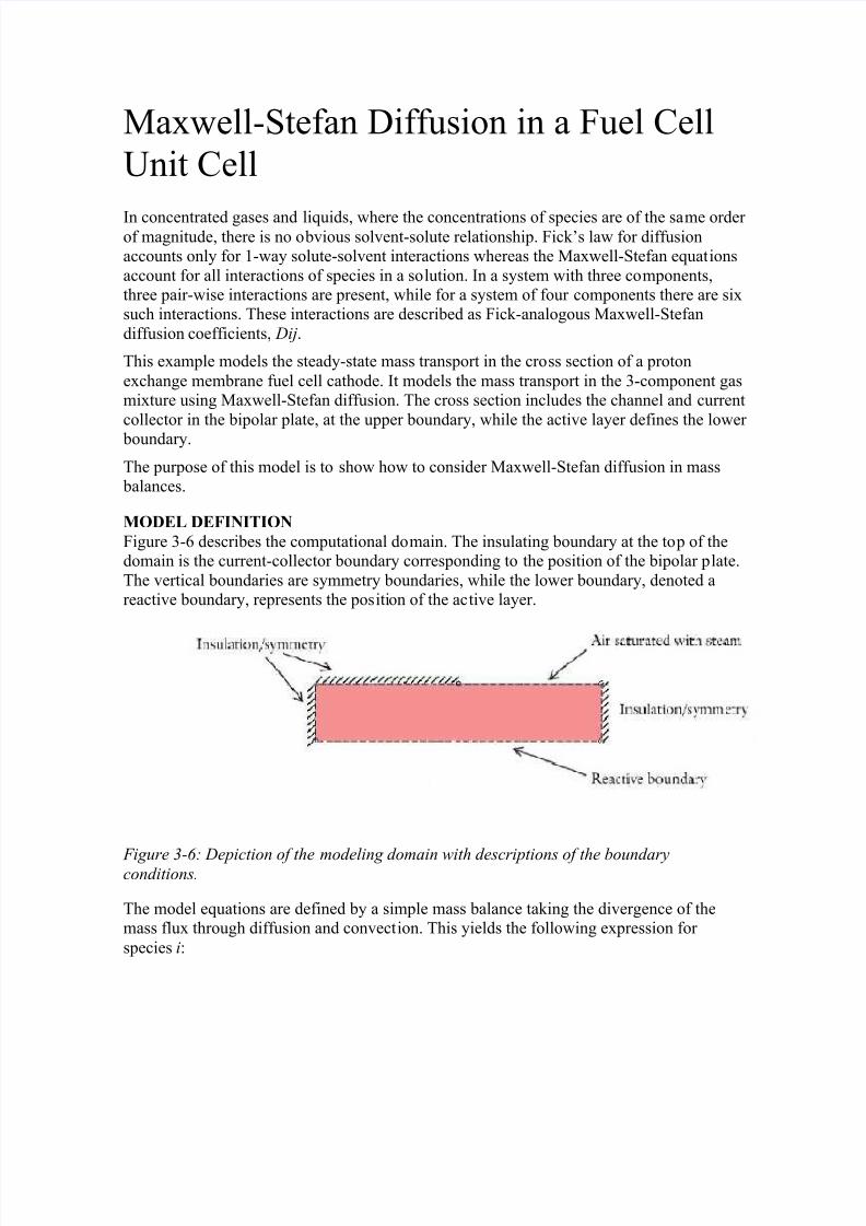
Figure 3-6 describes the computational domain. The insulating boundary at the top of thedomain is the current-collector boundary corresponding to the position of the bipolar plate.

The vertical boundaries are symmetry boundaries, while the lower boundary, denoted areactive boundary, represents the position of the active layer.

F igure 3-6: Depiction of the modeling domain with descriptions of the boundaryconditions.

The model equations are defined by a simple mass balance taking the divergence of themass flux through diffusion and convection. This yields the following expression for

species i:



where M denotes the total molar mass of the mixture (kg/mol), M j gives the molar mass of species j (kg/mol), and j is the mass fraction of species j. M can also be expressed in termsof the mass fractions, j. The symmetric diffusivities are strongly dependent on the

composition and are given by these expressions (see Ref. 2 and Ref. 3):

where xj is the mol fraction of species j (which can be expressed in terms of the mass

fractions j), and Dij is the Maxwell-Stefan diffusivities (m2/s). Additional entries of the

symmetric diffusivities are constructed by permutation of the indices, that is, D12 = D21.The Maxwell-Stefan diffusivities can be described with an empirical equation (Ref. 4) based on the kinetic gas theory:

where k is a constant with the value 3.16e-8, T is the temperature (K), p denotes the pressure (Pa), ni equals the molar diffusion volume (m3/mol) of species i, and M i is

the molar mass of species i. The molar diffusion volumes are given in Table 3-1 (Ref. 1).



At the reactive boundary (the electrode), the flux of oxygen is

wheren

j represents the mass flux of j, and ic is the reaction current given by the Tafelexpression:

Here Sa denotes the specific surface area (m2/m3), and is the thickness of the active layer (m). In the Tafel equation, F denotes Faraday¶s number (A· s/mol), R is the gas constant

(J/(mol·K)), T represents the temperature (K), i0 denotes the exchange current density(A/m2), and is the overpotential (V). The subscript 0 in the mass fraction for oxygen

represents the reference state.

Similarly, the flux of water is

where t H2O is the transport number for water (that is, the number of water molecules

dragged with each proton migrating through the membrane).

At the reactive boundary there is no flux of nitrogen gas because it does not take part in the

reactions. This boundary condition results in zero total flux of nitrogen in the entire

subdomain at steady state. Included this fact in the model by specifying the subdomain gasvelocity according to



At the inlet, a fixed composition is applied. This model uses a composition of air saturated

with steam at 80 oC as according to the following table (Ref. 1).

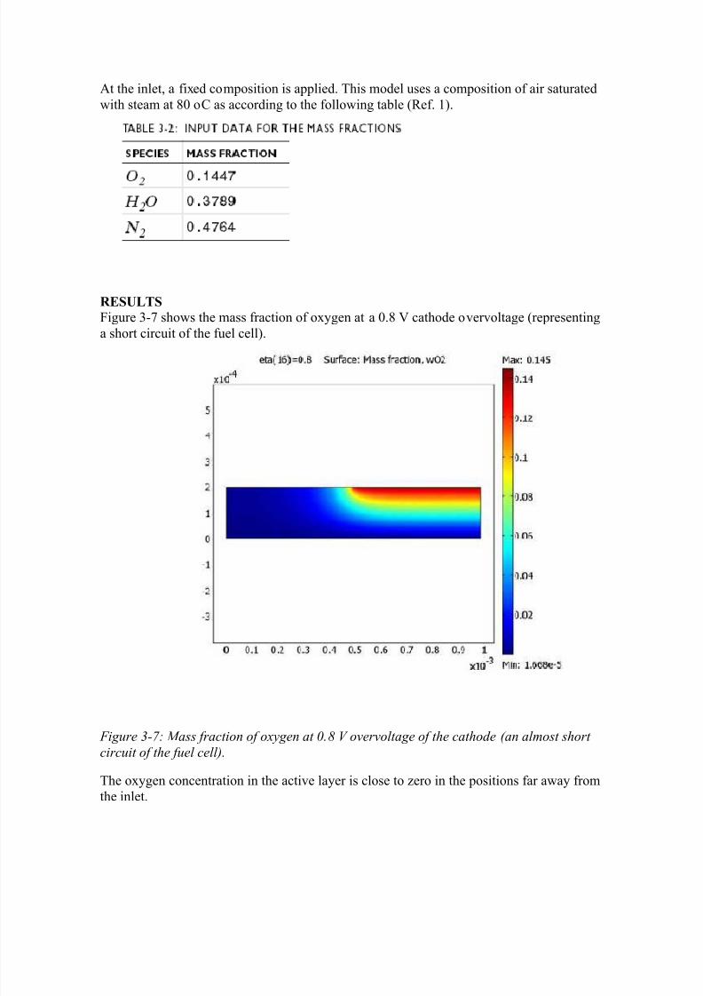
R ESULTS Figure 3-7 shows the mass fraction of oxygen at a 0.8 V cathode overvoltage (representing

a short circuit of the fuel cell).

F igure 3-7: M ass fraction of oxygen at 0.8 V overvoltage of the cathode (an almost short

circuit of the fuel cell).

The oxygen concentration in the active layer is close to zero in the positions far away from

the inlet.



The large variation in concentration has a direct influence on the value of the diffusion

coefficients for oxygen and the other involved species, nitrogen and water.

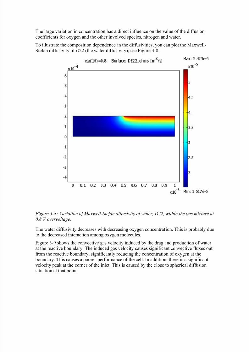
To illustrate the composition dependence in the diffusivities, you can plot the Maxwell-

Stefan diffusivity of D22 (the water diffusivity); see Figure 3-8.

F igure 3-8: Variation of M axwell-Stefan diffusivity of water, D22, within the gas mixture at 0.8 V overvoltage.

The water diffusivity decreases with decreasing oxygen concentration. This is probably dueto the decreased interaction among oxygen molecules.

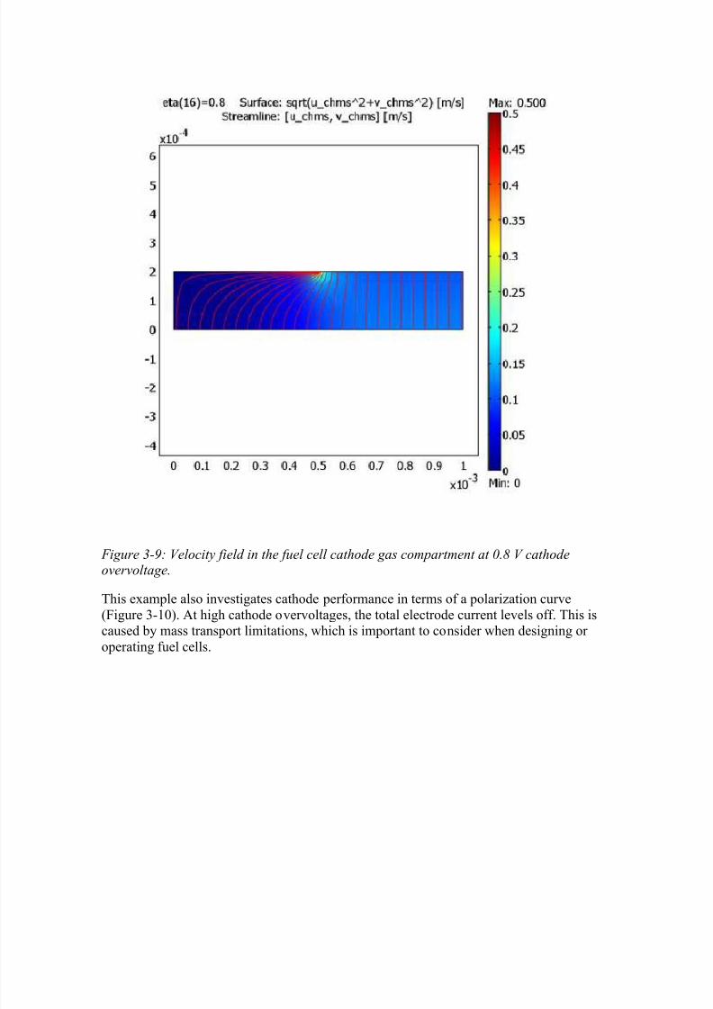
Figure 3-9 shows the convective gas velocity induced by the drag and production of water

at the reactive boundary. The induced gas velocity causes significant convective fluxes outfrom the reactive boundary, significantly reducing the concentration of oxygen at the boundary. This causes a poorer performance of the cell. In addition, there is a significant

velocity peak at the corner of the inlet. This is caused by the close to spherical diffusionsituation at that point.



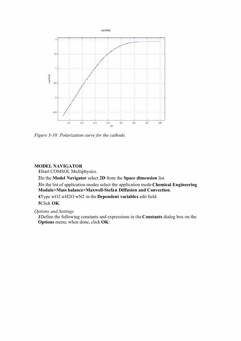
F igure 3-10: Polarization curve for the cathode.

MODEL NAVIGATOR 1Start COMSOL Multiphysics.

2In the Model Navigator select 2D from the Space dimension list.3In the list of application modes select the application mode Chemical Engineering

Module>Mass balance>Maxwell-Stefan Diffusion and Convection.

4Type wO2 wH2O wN2 in the Dependent variables edit field.

5Click OK .

O ptions and Settings

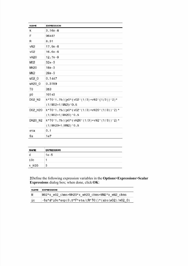
1Define the following constants and expressions in the Constants dialog box on theOptions menu; when done, click OK :



2Define the following expression variables in the Options>Expressions>Scalar

Expressions dialog box; when done, click OK :



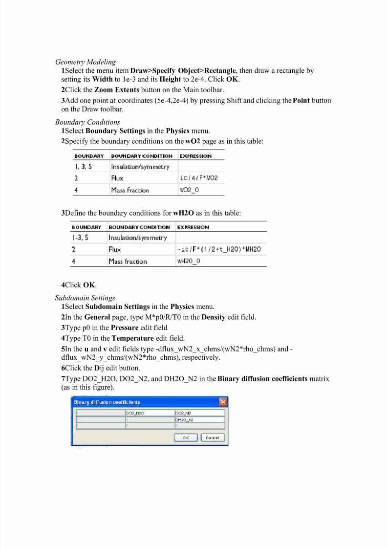
Geometry M odeling 1Select the menu item Draw>Specify Object>R ectangle, then draw a rectangle bysetting its Width to 1e-3 and its Height to 2e-4. Click OK .

2Click the Zoom Extents button on the Main toolbar.

3Add one point at coordinates (5e-4,2e-4) by pressing Shift and clicking the Point buttonon the Draw toolbar.

Boundary Conditions 1Select Boundary Settings in the Physics menu.

2Specify the boundary conditions on the wO2 page as in this table:

3Define the boundary conditions for wH2O as in this table:

4Click OK .

Subdomain Settings 1Select Subdomain Settings in the Physics menu.

2In the General page, type M*p0/R/T0 in the Density edit field.

3Type p0 in the Pressure edit field

4Type T0 in the Temperature edit field.

5In the u and v edit fields type -dflux_wN2_x_chms/(wN2*rho_chms) and -dflux_wN2_y_chms/(wN2*rho_chms), respectively.

6Click the Dij edit button.

7Type DO2_H2O, DO2_N2, and DH2O_N2 in the Binary diffusion coefficients matrix(as in this figure).



8Click the tabs for each species and type MO2, MH2O and MN2 in the corresponding

Molecular weight edit fields.

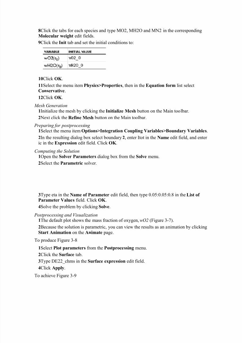
9Click the Init tab and set the initial conditions to:

10Click OK .

11Select the menu item Physics>Properties, then in the Equation form list selectConservative.

12Click OK .

M esh Generation 1Initialize the mesh by clicking the Initialize Mesh button on the Main toolbar.

2 Next click the R efine Mesh button on the Main toolbar.

Preparing for postprocessing 1Select the menu item Options>Integration Coupling Variables>Boundary Variables.

2In the resulting dialog box select boundary 2, enter Itot in the Name edit field, and enter ic in the Expression edit field. Click OK .

Computing the Solution 1Open the Solver Parameters dialog box from the Solve menu.

2Select the Parametric solver.

3Type eta in the Name of Parameter edit field, then type 0.05:0.05:0.8 in the List of Parameter Values field. Click OK .

4Solve the problem by clicking Solve.

Postprocessing and Visualization 1The default plot shows the mass fraction of oxygen, wO2 (Figure 3-7).

2Because the solution is parametric, you can view the results as an animation by clicking

Start Animation on the Animate page.

To produce Figure 3-8

1Select Plot parameters from the Postprocessing menu.

2Click the Surface tab.

3Type DE22_chms in the Surface expression edit field.

4Click Apply.

To achieve Figure 3-9



1Go to the Surface page and enter sqrt(u_chms^2+v_chms^2) in the Expression field.

2In the Streamline page, type u_chms and v_chms in the edit fields for x- and y

components, respectively. Select the Streamline plot check box.

3Select Specify start point coordinates in the Streamline start points section of thedialog box, then type linspace(1e-5,0.99e-5,25) into the x: edit field and zeros(1,25) into

the y: edit field.

4Click OK .

Finally, generate Figure 3-10 with these steps:

1Select the menu item Postprocessing>Domain Plot Parameters.

2In the Point page, type log10(Itot) in the Expression edit field.

3Select point 1, then click OK .

Maxwell Ingles

Documents

Transcript of Maxwell Ingles