The propagation of industrial business cyclesThe propagation of industrial business cycles Maximo...

The propagation of industrial business cycles�

Maximo Camachoy

Universidad de Murcia

[email protected]

Danilo Leiva-Leon

Bank of Canada

[email protected]

June 18, 2014

Abstract

This paper examines the business cycle linkages that propagate industry-speci�c business

cycle shocks throughout the economy in a way that (sometimes) generate aggregated cycles.

The transmission of sectorial business cycles is modelled through a multivariate Markov-

switching model, which is estimated by Gibbs sampling. Based on nonparametric density

estimation approaches, we �nd that the number and location of modes in the distribution of

industrial dissimilarities change over the business cycle. There is a relatively stable trimodal

pattern during expansionary and recessionary phases characterized by highly, moderately

and lowly synchronized industries. However, during phase changes, the density mass spreads

out from the central part to the higher end of lowly synchronized industries.

Keywords: Business Cycles, Output Growth, Time Series.

JEL Classi�cation: E32, C22, E27

�We are thankful to Gabriel Perez Quiros for their comments. M. Camacho acknowledges support

from project ECO2010-19830. All remaining errors are our responsibility. The views in this paper are

those of the authors and do not represent the views of the Bank of Canada.yCorresponding Author: Universidad de Murcia, Facultad de Economia y Empresa, Departamento de

Metodos Cuantitativos para la Economia y la Empresa, 30100, Murcia, Spain. E-mail: [email protected].

1

1 Introduction

In practice, people do not know the state of the business cycle, which is especially uncertain

around the turning points. This could be because �the state of the economy�depends on the

behavior of many interdependent industries that do not necessarily boom when the aggregate

economy is prosperous and bust when the economy is in recession in a synchronous manner.

Accordingly, although the aggregate business cycle could be described at a macro level as a series

of distinct recession and expansion phases, it could never be understood at that level. Although

recessions are not all alike, some lessons can be learnt regarding their propagation when tracking

the micro foundations of cycles through a variety of interconnected market dynamics at industry

levels.

The main purpose of this paper is to understand when microeconomic idiosyncratic business

cycle shocks lead to aggregate �uctuations, which industries manifest the �rst signs of the phase

changes and how the interconnections across industries lead to cascade e¤ects that propagate the

idiosyncratic shocks to the rest of the economy. Our analysis contributes to several strands of the

existing literature. First, Gabaix (2011) and Acemoglu, Carvalho, Ozdaglar and Tahbaz-Salehi

(2012) postulate that when there exist signi�cant asymmetries in the roles that industries play

as suppliers to others, idiosyncratic �rm-level shocks can explain an important part of aggregate

movements. Foerster, Sarte and Watson (2011) show that the role of sectorial shocks increased

considerably after the Great Moderation. We complement these analyses by focusing on the

transmission of shocks over the distinct business cycle phases.

Second, the sharp downturn in the economy experienced in 2008 and the subsequent jobless

recovery increased concerns for security for asset holders (Malmendier and Nagel, 2011) and for

people seeking their work (Urquhart, 1981). Our analysis could help investors, who can reduce

asset risk and workers, who can improve job security, by shifting to less sensitive industries

to the aggregate cycle in bad times. For this purpose, we characterize salient features of the

propagation of industrial business cycles.

Third, although the business cycle analysis has largely focused on national-level phases,

there is a growing interest on state-level data (Owyang, Piger and Wall, 2005, and Hamilton

and Owyang, 2012) and on city-level data (Owyang, Piger, Wall and Wheeler, 2008). The

former authors �nd that the disparities in regional business cycles can partially be attributed

to di¤erences in the industrial composition of the regions and the latter authors �nd that the

low-phase growth is related only to the relative importance of manufacturing. Undoubtedly,

2

these analyses could be complemented by examining the business cycle at industry level.

In spite of its interest in the literature, little attention has been paid to analyze the business

cycle dynamics at the industry level. Not being exhaustive, some examples are the following.

Christiano and Fitzgerald (1998) gauge the extent of co-movement across a range of disaggre-

gated sector categories and the total by computing the square of the correlation between their

business cycle components in hours worked, which are the outcome of band-pass �lters. Carlino

and DeFina (2004) focus on the analysis of growth cycles by examining the pairwise correlation

between the sectorial cycles in band-pass �ltered employment. Recently, Goodman and Mance

(2011) analyze the percent change in industry employment data during recessions, as determined

by the National Bureau of Economic Research (NBER).

One important drawback of these analyses is that they rely on static measures. Therefore,

the changes over time can only be captured by splitting the samples into sub-periods. The

problem of these approaches is that they provide pictures of the cycle linkages that rely on

speci�c date breaks, whose location is sometimes controversial. To our knowledge, no attention

has been paid to examine the time-varying dynamics of these interactions, which is crucial to

understand the transmission of business cycle shocks across industries. To plug such a gap, this

paper aims at establishing a rigorous procedure to characterize the propagation of business cycle

shocks at the industry level.

For this purpose, this paper uses an extension of the Markov-switching model of Hamilton

(1989) that computes inferences of the industry cycles and characterize the evolution of the

interactions across their cycles by combining the framework developed by Bengoechea, Camacho

and Perez Quiros (2006) and Leiva-Leon (2014). In particular, each of the industrial cycles is

viewed as a continuous-valued Markov-switching variable whose transition between two distinct

phases de�nes the states of its business cycles. The synchronization of two industries in a

bivariate speci�cation is viewed as a time-varying combination between two extreme cases: two

independent Markov processes, which refers to completely independent industries, and a unique

Markov process shared by both industries, which refers to perfect synchronization. The shifts

between these extreme regimes is governed by the outcome of an unobserved Markov chain.

By means of purely statistical techniques, such as non-parametric density estimation and

bootstrap multimodality tests, the number of modes in the time-varying distributions of pair-

wise business cycle dissimilarities is tested. In our context, this is useful to uncover distinct

business cycle dynamics for di¤erent population subgroups of industries and to assess how these

3

subgroups evolve across the distinct phases of the business cycle. Finally, multidimensional

scaling techniques are used to understand the formation of these subgroups and their intra-

distribution transitional dynamics.

Among many others, in our analysis we report two major �ndings. First, we �nd that the US

business cycle at micro level is a more elusive phenomenon than we might have expected at macro

level. Whilst some industries seem to �stick together�and show business cycle experiences that

are similar to those of the nation, there are many which do not. The distribution of the ergodic

business cycle dissimilarities has a big hump at the high-end representing the industries that are

less sensitive to the national business cycle. However, it also shows a prominent middle mass

and a smaller low-end hump representing those industries typically considered as procyclical.

Second, we detect a thought-provoking recurrent business cycle pattern. Over the last three

decades, a salient characteristic of the US cycle dynamics is that the distribution of business

cycle dissimilarities across industries shifts over time. During expansions and recessions, the

distribution is characterized by three clusters of highly, moderately, and lowly synchronized

industries, yielding a trimodal distribution. However, during the periods of business cycle phase

shifts or turning points, the middle-synchronized industries enjoyed downward synchronization

mobility and vanish into the lowly synchronized class, yielding a bimodal distribution. Once

the transitions have ended, the trend is reversed and the economy stabilizes in the new business

cycle phase. We postulate that the di¤erences in the structure of the industrial labour markets

could cause this transitional dynamics.

The structure of this paper is organized as follows. Section 2 describes the framework used to

compute inferences on the industrial business cycle dynamics. Section 3 presents the empirical

results. Section 4 concludes and proposes some lines of future research.

2 Assessing the industrial business cycles

Two things are required to study the comovement across industries over the business cycle: a

measure of economic activity in the industries and a precise de�nition of their business cycles.

In this paper, the economic activity at date t in a given sector is measured by the annual growth

rates of total employees in the sector. The de�nition of business cycles relies on the recognized

empirical fact that although the series of employment present trends they are not monotonic

curves, but rather exhibit sequences of upturns and downturns that agree with their business

4

cycles phases. During the periods known as recessions, the value of the employment growth rates

are usually lower (and sometimes negative) than during the periods of expansion. A natural

approach to model this particular nonlinear dynamic behavior is the regime switching model

proposed by Hamilton (1989)

2.1 Univariate model

Following Hamilton (1989), we assume that the switching mechanism of the k-th sector�s em-

ployment growth at time t, yk;t, is controlled by an unobservable state variable, sk;t. Owyang,

Piger, and Wall (2005) specify a simple switching model that captures this nonlinear dynamics

yk;t = �sk;t + "k;t; (1)

where the growth rate of employment in sector k at date t has mean �sk;t = �k0 + �k1sk;t,

which is allowed to switch between two distinct regimes. At time t, one can label sk;t = 0 as

expansions and sk;t = 1 as recessions. Deviations from this mean growth rate are created by "k;t,

which is an i:i:d: Gaussian stochastic disturbance with mean zero and variance �2k. Therefore,

employment is expected to exhibit high (usually positive) growth rates in expansions and low

(usually negative) growth rates in recessions. The variable sk;t is assumed to evolve according

to �rst-order Markov chain, whose transition probabilities are de�ned by

p (sk;t = jkjsk;t�1 = ik; st�2 = rk; :::; eyk;t�1) = p (sk;t = jkjsk;t�1 = ik) = pkij ; (2)

where i; j = 1; 2, and eyk;t = (yk;t; ; yk;t�1; ::::)0.2.2 Bivariate model

Although univariate Markov-switching models provide information about the timing of the

regime changes, they are inappropriate for drawing inferences about the synchronization of

business cycles. Camacho and Perez Quiros (2006) show that the business cycle analyses based

on univariate processes are biased to show relatively low values of business cycle synchronization.

Therefore, using univariate models would become particularly painful in the case of industries

that exhibit highly synchronized cycles.

Phillips (1991) shows that the univariate model can be slightly modi�ed to examine the

business cycle transmission in a two-sector setup. Let us assume that we are interested in

measuring the degree of business cycle synchronization between two industries a and b. In

5

this case, their employment growths are driven by two (possibly dependent) Markov-switching

processes, sa;t and sb;t, which share the statistical properties of the previous latent variable sk;t.

The bivariate state dependent model is given by

ya;t = �sa;t + "a;t;

yb;t = �sb;t + "b;t; (3)

where ("a;t; "b;t)0 is an identically and independently distributed bivariate Gaussian process with

zero mean and covariance matrix ab. To complete the dynamic speci�cation of the process, one

can de�ne a new state variable sab;t that characterizes the regime for date t in a way consistent

with the previous univariate speci�cation. The basic states of sab;t are

sab;t =

8>>>>>><>>>>>>:

1 if sa;t = 0 and sb;t = 0




; (4)

which encompasses all the possible combinations.

Bengoechea, Camacho and Perez Quiros (2006) postulate that this speci�cation allows for

two extreme kinds of interdependence between the business cycles of two industries. The �rst

case characterizes industries for which their individual business cycle �uctuations are completely

independent. The opposite case of perfect synchronization refers to the case in which both

industries share the state of the business cycle. In this case, their business cycles are generated

by the same state variable, so sa;t = sb;t. In empirical applications, the business cycles of two

industries usually exhibit an intermediate degree of synchronization that is located between

these two extreme possibilities in the sense of a weighted average. These authors consider that

the actual business cycle synchronization is �ab times the case of independence and (1� �ab)

times the case of perfect dependence, where 0 � �ab � 1. The weights �ab may be interpreted as

measures of business cycle desynchronization since they evaluate the proximity of their business

cycles to the case of complete independence. This suggests that an intuitive measure of business

cycle comovement is 1��ab. Using pairwise comparisons, the collection of 1��ab for each sector a

and b catches a glimpse of the business cycle synchronization across the collection of industries.

However, one important limitation of this approach is that the propagation throughout the

interconnected industries of business cycle shocks could only be examined by splitting the sample.

6

To overcome this drawback, Leiva-Leon (2014) suggests that independence and perfect de-

pendence constitute two distinct business cycle situations, with the shifts between these extreme

regimes governed by the outcome of an unobserved �rst-order Markov chain, vab;t, whose tran-

sition probabilities are given by

p (vab;t = jjvab;t�1 = i; st�2 = r; :::; eyab;t�1) = p (vab;t = jjvab;t�1 = i) = pabij ; (5)

where i; j = 1; 2, and eyab;t = (ya;t; ; ya;t�1; ::::; yb;t; yb;t�1; ::::)0. Here, the state variable vab;t

re�ects the actual state of the business cycle synchronization between industries a and b at

time t. In what follows, vab;t = 0 indicates that industries a and b have independent cycles

while vab;t = 1 indicates that their cycles are fully synchronized. Accordingly, p (vab;t = 0)

measures the probability of independent cycles. Within this framework, one can easily examine

the evolution of the intersectoral business cycle linkages by collecting p (vab;t = 0) for all a, b

and t.

2.3 Inferences

Collect the parameters that fully characterizes the model in a vector �. It is convenient to de�ne

a new state variable that governs the individual business cycles and its degree of synchronization

s�ab;t =

8>>>>>>>>>>>>>>>>>>><>>>>>>>>>>>>>>>>>>>:

1 if sa;t = 0, sb;t = 0, and vab;t = 0








; (6)

which also follows a �rst order Markov chain.1 Using an extended version of the procedure

described in Hamilton (1989), inferences on the business cycle states are calculated as a by-

product of an algorithm, which, in spirit, is similar to a Kalman �lter. Brie�y, the procedure is

based on the iterative application of the following two steps.

1The probabilities of occurrence of states 6 and 7 are zero by de�nition.

7

STEP 1: Computing the likelihoods. At time t, the method adds the observation yab;t =

(ya;t; yb;t)0 to eyab;t�1 and accepts as input the forecasting probabilities

p�s�ab;t = ijeyab;t�1; �� (7)

for i = 1; 2; :::; 8. In this case, the likelihood of yab;t is

fab (yab;tjeyab;t�1; �) = 8Xi=1

fab�ytjs�ab;t = i; eyab;t�1; �� p �s�ab;t = ijeyab;t�1; �� ; (8)

where fab (�) is the conditional Gaussian bivariate density function.

To perform inference, the joint probabilities can be obtained from the marginal probabilities

as

p�s�ab;t = ijeyab;t�1; �� = p (sab;t = jjvab;t = h; eyab;t�1; �) p (vab;t = hjeyab;t�1; �) ; (9)

with i = 1; :::; 8, j = 1; :::; 4 and h = 0; 1. The way on which the model computes inferences on

the four-state unobservable variable sab;t depends on the business cycle synchronization between

industries a and b. Suppose that each of these two industries follows independent regime-shifting

processes, i.e., vab;t = 0. Then, the four-state probability term of sab;t is

p (sab;t = jjvab;t = 0; eyab;t�1; �) = p (sa;t = jajeyab;t�1; �) p (sb;t = jbjeyab;t�1; �) ; (10)

with j = 1; :::; 4.

By contrast, if the two industries exhibit perfectly correlated business cycles, which occurs

when vab;t = 1, they could be represented by the same state variable since sa;t = sb;t. Therefore,

one can de�ne a new four-state variable &ab;t as in (4), where states 2 and 3 never occur and the

two industries share the cycle in states 1 and 4. In this case, the probability term is

p (sab;t = jjvab;t = 1; eyab;t�1; �) = p (&ab;t = jjeyab;t�1; �) ; (11)

with j = 1; :::; 4 and p (&ab;t = 2jeyab;t�1; �) = p (&ab;t = 3jeyab;t�1; �) = 0. The transition probabil-ities of &ab;t are

p (&ab;t = jj&ab;t�1 = i; &ab;t�2 = h; :::; eyab;t�1) = p (&ab;t = jj&ab;t�1 = i) = qabij : (12)

STEP 2: Updating the forecasting probabilities. Using the data up to time t, the optimal

8

inference on the state variables can be obtained in the following way

p (sk;t = jkjeyab;t; �) = fk (yk;tjsk;t = jk; eyab;t�1; �) p (sk;t = jkjeyab;t�1; �) =fk (yk;tjeyab;t�1; �) ;(13)p (vab;t = hjeyab;t; �) = fab (yab;tjvab;t = h; eyab;t�1; �) p (vab;t = hjeyab;t�1; �) =fab (yab;tjeyab;t�1; �) ;(14)

p (&ab;t = jjeyab;t; �) = fab (yab;tj&ab;t = j; eyab;t�1; �) p (&ab;t = jjeyab;t�1; �) =fab (yab;tjeyab;t�1; �) ;(15)p (sab;t = jjeyab;t; �) = fab (ytjsab;t = i; eyab;t�1; �) p (sab;t = jjeyab;t�1; �) =fab (ytjeyab;t�1; �) ; (16)where fk (�) is the conditional Gaussian univariate density function of industry jk, h = 1; 2,

j = 1; :::; 4, and k = a; b.

Finally, one can form the forecasts of how likely the processes are in period t+ 1, using the

observations up to date t. These forecasts can be computed by using the following expressions

p (sk;t+1 = jkjeyab;t; �) =1X

ik=0

p (sk;t = ikjeyab;t; �) pikjk ; (17)

p (vab;t+1 = hjeyab;t; �) =

1Xi=0

p (vab;t = ijeyab;t; �) pab;ij ; (18)

p (&ab;t+1 = jjeyab;t; �) =

4Xi=1

p (&ab;t = jjeyab;t; �) pij ; (19)

p (sab;t+1 = jjeyab;t; �) =

4Xi=1

p (sab;t = ijeyab;t; �) pab;ij : (20)

Then, the joint probabilities p�s�ab;t+1 = ijeyab;t; �� can be updated by using (9) and used in

computing the likelihood for the next period as described in the �rst step.

In the classical approach, the estimate of the parameters of the model is obtained by maximiz-

ing the likelihood function (8) by numerical optimization. In this context, performing inference

based on maximum likelihood becomes computationally cumbersome due to the complicated na-

ture of the joint likelihood function. In Appendix A, we describe a multi-move Gibbs-sampling

method that makes the Bayesian analysis approach easy to implement. Skipping the details,

both the parameters of the model, �, and the Markov-switching variable, es�ab;T = s�ab;1; :::; s�ab;T ,are treated as random variables. This Monte Carlo Markov chain method is achieved by sequen-

tially generating a realization �j from the distribution of �jeyab;T ; es�j�1ab;T followed by a realization

of es�jab;T from the distribution of es�ab;T jeyab;T ; �j . Thus, the marginal distributions of the statevariables and the parameters of the model can be approximated by the empirical distribution of

the simulated values. The descriptive statistics regarding the sample posterior distributions are

9

then based on 12; 000 draws, where the �rst 2; 000 draws are discarded to mitigate the e¤ect of

initial conditions.

3 Empirical analysis

3.1 Data description

The data used to measure the industry level business cycles are the seasonally adjusted, year-

over-year growth rates of employment from the Current Employment Statistics survey. To

classify, we follow the three-digit industry using the North American Industry Classi�cation

System (NAICS). The e¤ective sample period is 1991:01 to 2013:05 and the list of 86 industries

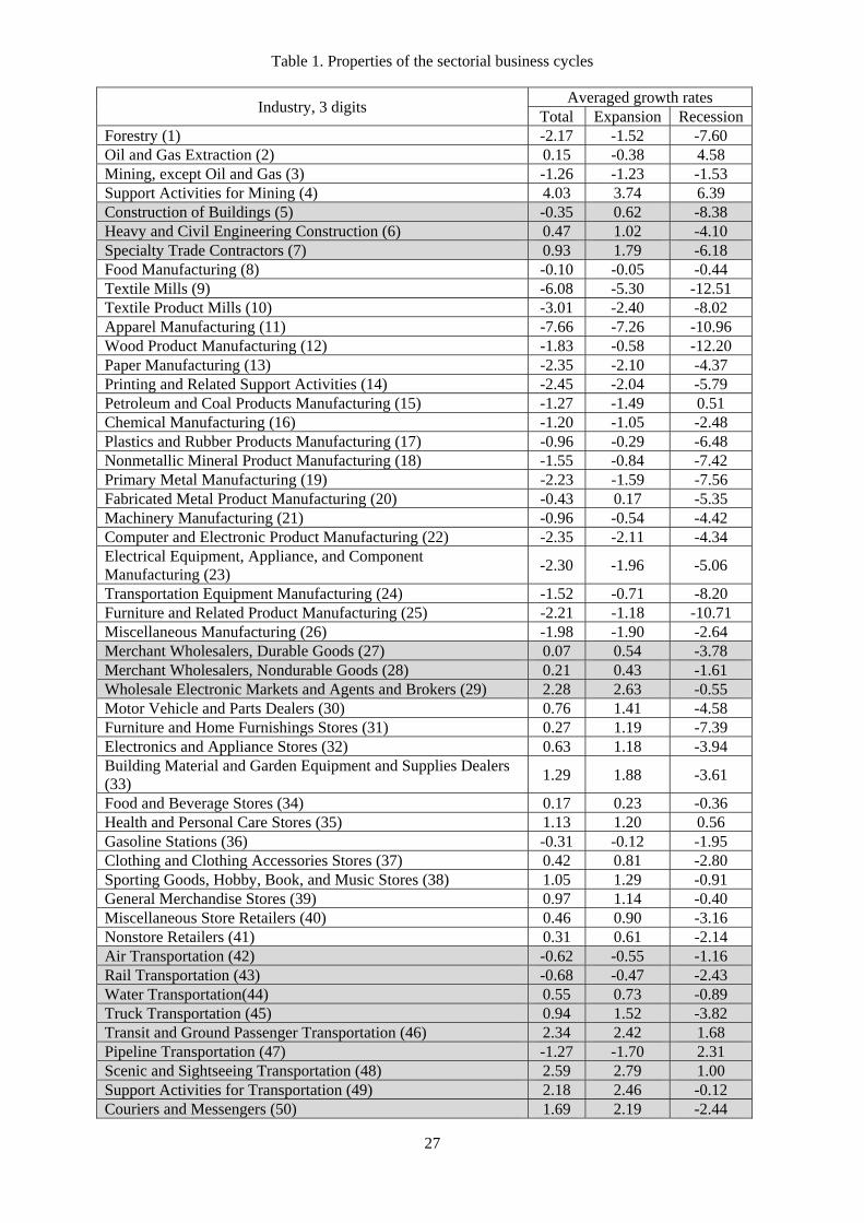
included in the analysis appears in Table 1.2

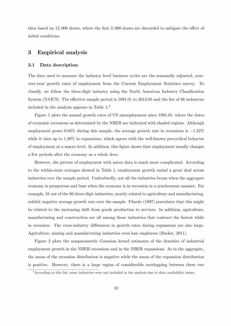
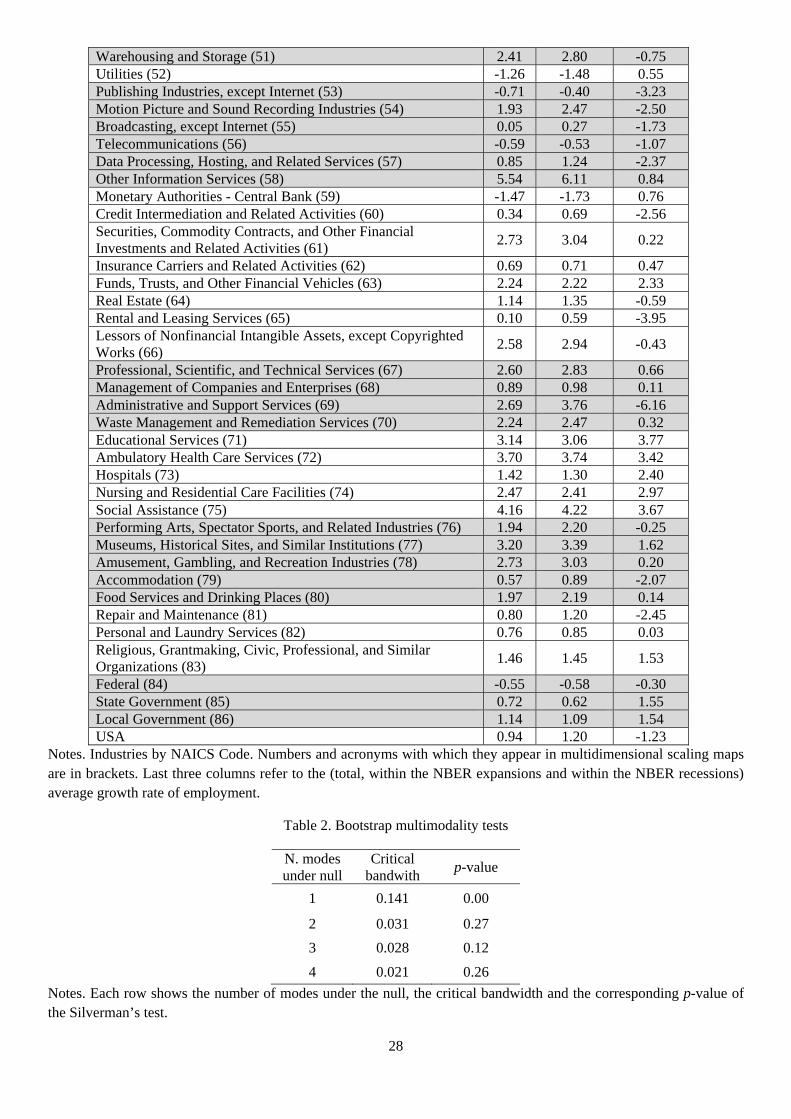
Figure 1 plots the annual growth rates of US unemployment since 1991:01, where the dates

of economic recessions as determined by the NBER are indicated with shaded regions. Although

employment grows 0:94% during this sample, the average growth rate in recessions is �1:22%

while it rises up to 1:20% in expansions, which agrees with the well-known procyclical behavior

of employment at a macro level. In addition, this �gure shows that employment usually changes

a few periods after the economy as a whole does.

However, the picture of employment with micro data is much more complicated. According

to the within-state averages showed in Table 1, employment growth varied a great deal across

industries over the sample period. Undoubtedly, not all the industries boom when the aggregate

economy is prosperous and bust when the economy is in recession in a synchronous manner. For

example, 31 out of the 86 three-digit industries, mostly related to agriculture and manufacturing,

exhibit negative average growth rate over the sample. Filardo (1997) postulates that this might

be related to the increasing shift from goods production to services. In addition, agriculture,

manufacturing and construction are all among those industries that contract the fastest while

in recession. The cross-industry di¤erences in growth rates during expansions are also large.

Agriculture, mining and manufacturing industries even lose employees (Barker, 2011).

Figure 2 plots the nonparametric Gaussian kernel estimates of the densities of industrial

employment growth in the NBER recessions and in the NBER expansions. As in the aggregate,

the mean of the recession distribution is negative while the mean of the expansion distribution

is positive. However, there is a large region of considerable overlapping between these two

2According to this list, some industries were not included in the analysis due to data availability issues.

10

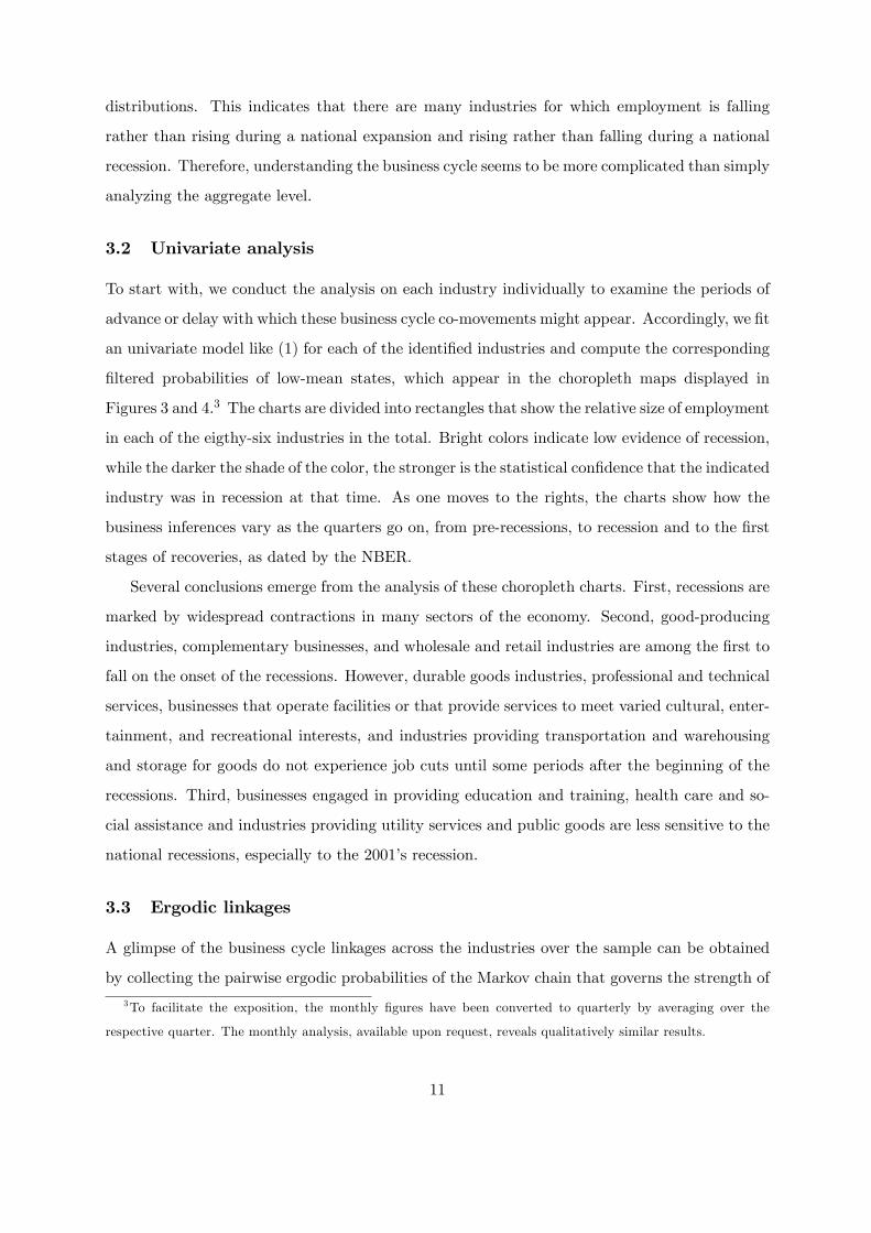
distributions. This indicates that there are many industries for which employment is falling

rather than rising during a national expansion and rising rather than falling during a national

recession. Therefore, understanding the business cycle seems to be more complicated than simply

analyzing the aggregate level.

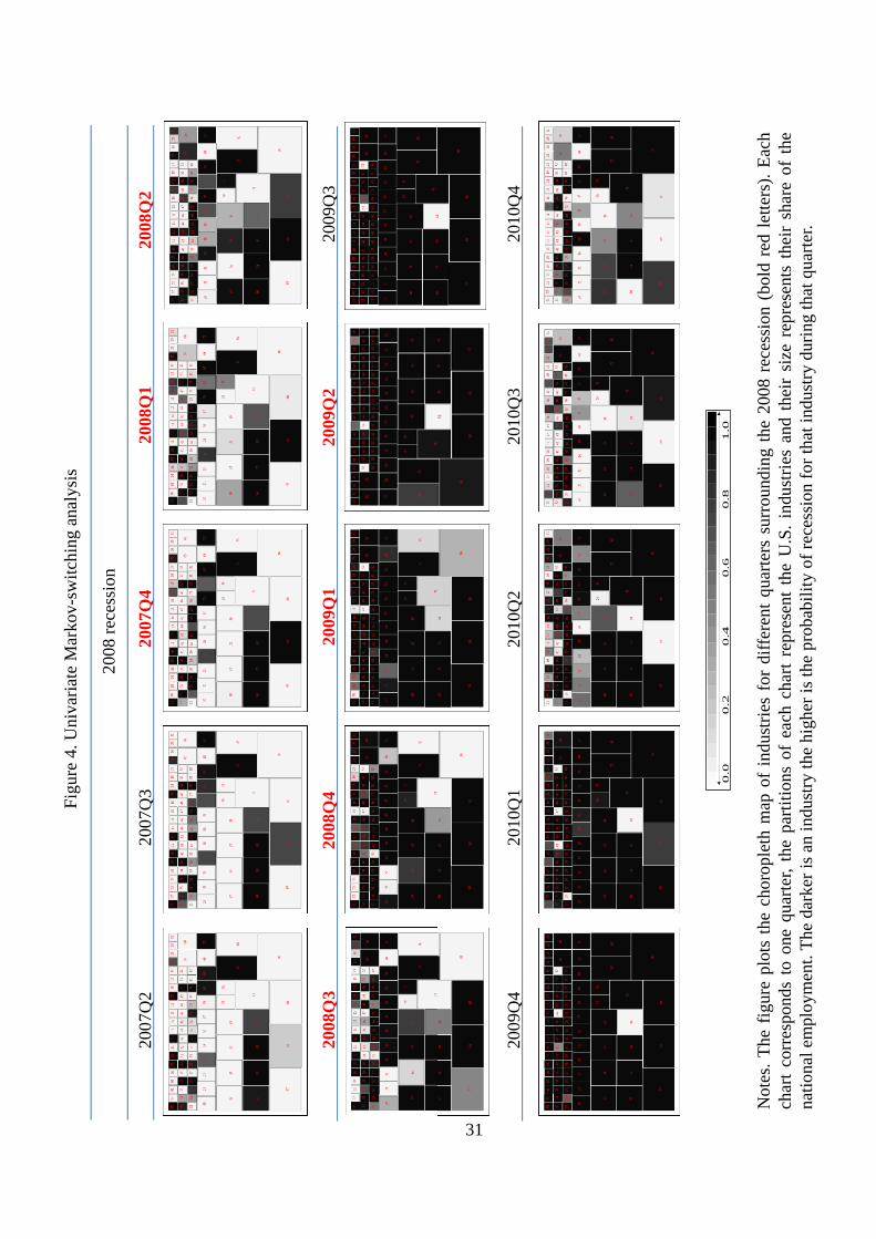
3.2 Univariate analysis

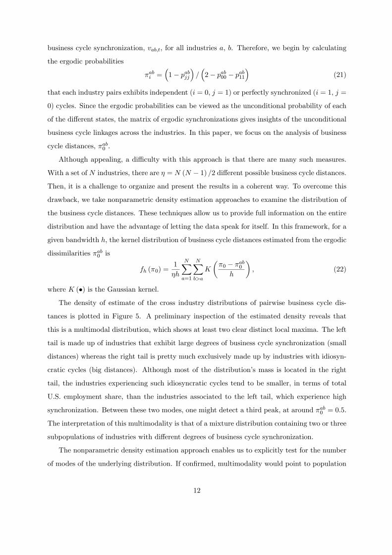
To start with, we conduct the analysis on each industry individually to examine the periods of

advance or delay with which these business cycle co-movements might appear. Accordingly, we �t

an univariate model like (1) for each of the identi�ed industries and compute the corresponding

�ltered probabilities of low-mean states, which appear in the choropleth maps displayed in

Figures 3 and 4.3 The charts are divided into rectangles that show the relative size of employment

in each of the eigthy-six industries in the total. Bright colors indicate low evidence of recession,

while the darker the shade of the color, the stronger is the statistical con�dence that the indicated

industry was in recession at that time. As one moves to the rights, the charts show how the

business inferences vary as the quarters go on, from pre-recessions, to recession and to the �rst

stages of recoveries, as dated by the NBER.

Several conclusions emerge from the analysis of these choropleth charts. First, recessions are

marked by widespread contractions in many sectors of the economy. Second, good-producing

industries, complementary businesses, and wholesale and retail industries are among the �rst to

fall on the onset of the recessions. However, durable goods industries, professional and technical

services, businesses that operate facilities or that provide services to meet varied cultural, enter-

tainment, and recreational interests, and industries providing transportation and warehousing

and storage for goods do not experience job cuts until some periods after the beginning of the

recessions. Third, businesses engaged in providing education and training, health care and so-

cial assistance and industries providing utility services and public goods are less sensitive to the

national recessions, especially to the 2001�s recession.

3.3 Ergodic linkages

A glimpse of the business cycle linkages across the industries over the sample can be obtained

by collecting the pairwise ergodic probabilities of the Markov chain that governs the strength of

3To facilitate the exposition, the monthly �gures have been converted to quarterly by averaging over the

respective quarter. The monthly analysis, available upon request, reveals qualitatively similar results.

11

business cycle synchronization, vab;t, for all industries a, b. Therefore, we begin by calculating

the ergodic probabilities

�abi =�1� pabjj

�=�2� pab00 � pab11

�(21)

that each industry pairs exhibits independent (i = 0; j = 1) or perfectly synchronized (i = 1, j =

0) cycles. Since the ergodic probabilities can be viewed as the unconditional probability of each

of the di¤erent states, the matrix of ergodic synchronizations gives insights of the unconditional

business cycle linkages across the industries. In this paper, we focus on the analysis of business

cycle distances, �ab0 .

Although appealing, a di¢ culty with this approach is that there are many such measures.

With a set of N industries, there are � = N (N � 1) =2 di¤erent possible business cycle distances.

Then, it is a challenge to organize and present the results in a coherent way. To overcome this

drawback, we take nonparametric density estimation approaches to examine the distribution of

the business cycle distances. These techniques allow us to provide full information on the entire

distribution and have the advantage of letting the data speak for itself. In this framework, for a

given bandwidth h, the kernel distribution of business cycle distances estimated from the ergodic

dissimilarities �ab0 is

fh (�0) =1

�h

NXa=1

NXb>a

K

��0 � �ab0

h

�; (22)

where K (�) is the Gaussian kernel.

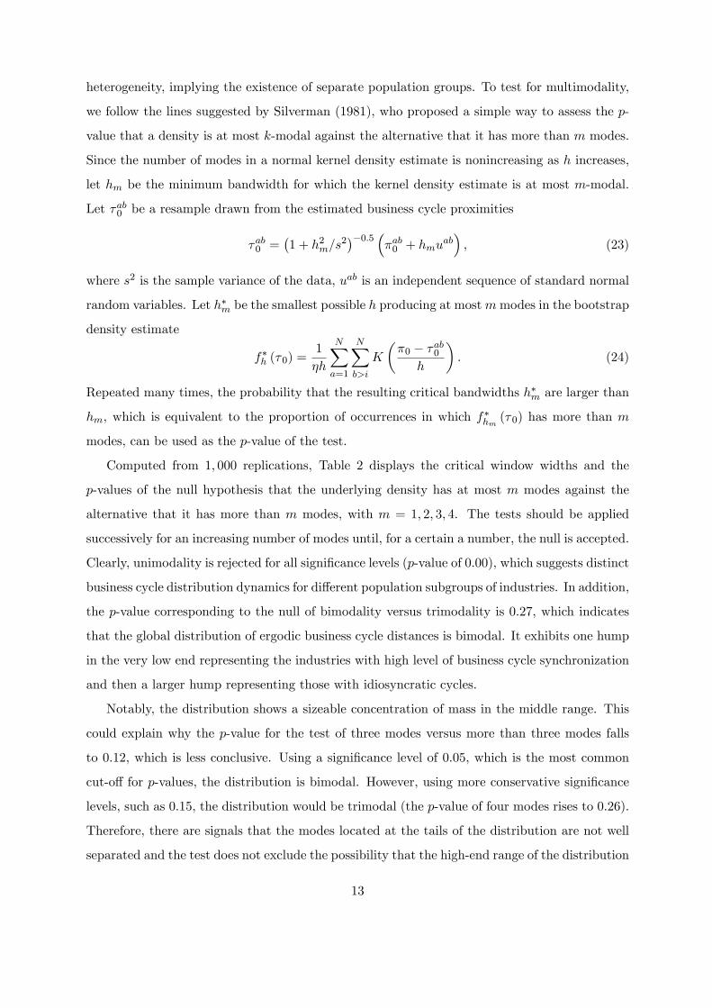
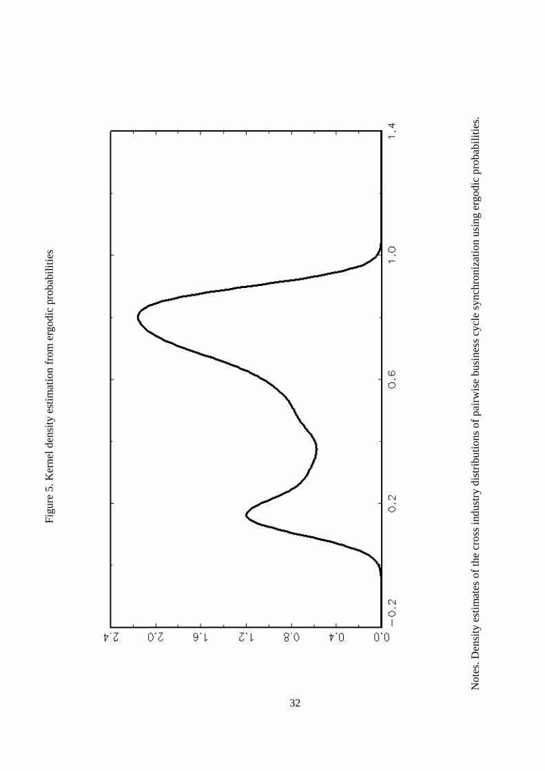
The density of estimate of the cross industry distributions of pairwise business cycle dis-

tances is plotted in Figure 5. A preliminary inspection of the estimated density reveals that

this is a multimodal distribution, which shows at least two clear distinct local maxima. The left

tail is made up of industries that exhibit large degrees of business cycle synchronization (small

distances) whereas the right tail is pretty much exclusively made up by industries with idiosyn-

cratic cycles (big distances). Although most of the distribution�s mass is located in the right

tail, the industries experiencing such idiosyncratic cycles tend to be smaller, in terms of total

U.S. employment share, than the industries associated to the left tail, which experience high

synchronization. Between these two modes, one might detect a third peak, at around �ab0 = 0:5.

The interpretation of this multimodality is that of a mixture distribution containing two or three

subpopulations of industries with di¤erent degrees of business cycle synchronization.

The nonparametric density estimation approach enables us to explicitly test for the number

of modes of the underlying distribution. If con�rmed, multimodality would point to population

12

heterogeneity, implying the existence of separate population groups. To test for multimodality,

we follow the lines suggested by Silverman (1981), who proposed a simple way to assess the p-

value that a density is at most k-modal against the alternative that it has more than m modes.

Since the number of modes in a normal kernel density estimate is nonincreasing as h increases,

let hm be the minimum bandwidth for which the kernel density estimate is at most m-modal.

Let �ab0 be a resample drawn from the estimated business cycle proximities

�ab0 =�1 + h2m=s

2��0:5 �

�ab0 + hmuab�; (23)

where s2 is the sample variance of the data, uab is an independent sequence of standard normal

random variables. Let h�m be the smallest possible h producing at mostmmodes in the bootstrap

density estimate

f�h (�0) =1

�h

NXa=1

NXb>i

K

��0 � �ab0

h

�: (24)

Repeated many times, the probability that the resulting critical bandwidths h�m are larger than

hm, which is equivalent to the proportion of occurrences in which f�hm (�0) has more than m

modes, can be used as the p-value of the test.

Computed from 1; 000 replications, Table 2 displays the critical window widths and the

p-values of the null hypothesis that the underlying density has at most m modes against the

alternative that it has more than m modes, with m = 1; 2; 3; 4. The tests should be applied

successively for an increasing number of modes until, for a certain a number, the null is accepted.

Clearly, unimodality is rejected for all signi�cance levels (p-value of 0.00), which suggests distinct

business cycle distribution dynamics for di¤erent population subgroups of industries. In addition,

the p-value corresponding to the null of bimodality versus trimodality is 0:27, which indicates

that the global distribution of ergodic business cycle distances is bimodal. It exhibits one hump

in the very low end representing the industries with high level of business cycle synchronization

and then a larger hump representing those with idiosyncratic cycles.

Notably, the distribution shows a sizeable concentration of mass in the middle range. This

could explain why the p-value for the test of three modes versus more than three modes falls

to 0:12, which is less conclusive. Using a signi�cance level of 0:05, which is the most common

cut-o¤ for p-values, the distribution is bimodal. However, using more conservative signi�cance

levels, such as 0:15, the distribution would be trimodal (the p-value of four modes rises to 0:26).

Therefore, there are signals that the modes located at the tails of the distribution are not well

separated and the test does not exclude the possibility that the high-end range of the distribution

13

could be split into two subgroups.

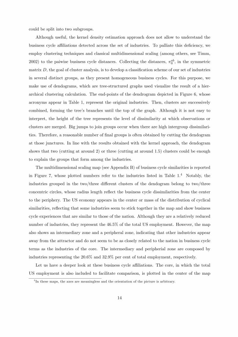
Although useful, the kernel density estimation approach does not allow to understand the

business cycle a¢ liations detected across the set of industries. To palliate this de�ciency, we

employ clustering techniques and classical multidimensional scaling (among others, see Timm,

2002) to the paiwise business cycle distances. Collecting the distances, �ab0 , in the symmetric

matrix D, the goal of cluster analysis, is to develop a classi�cation scheme of our set of industries

in several distinct groups, as they present homogeneous business cycles. For this purpose, we

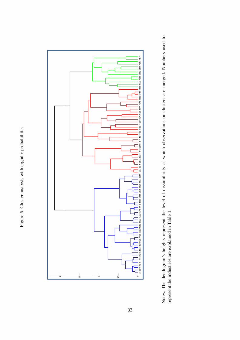
make use of dendograms, which are tree-structured graphs used visualize the result of a hier-

archical clustering calculation. The end-points of the dendrogram depicted in Figure 6, whose

acronyms appear in Table 1, represent the original industries. Then, clusters are successively

combined, forming the tree�s branches until the top of the graph. Although it is not easy to

interpret, the height of the tree represents the level of dissimilarity at which observations or

clusters are merged. Big jumps to join groups occur when there are high intergroup dissimilari-

ties. Therefore, a reasonable number of �nal groups is often obtained by cutting the dendogram

at those junctures. In line with the results obtained with the kernel approach, the dendogram

shows that two (cutting at around 2) or three (cutting at around 1:5) clusters could be enough

to explain the groups that form among the industries.

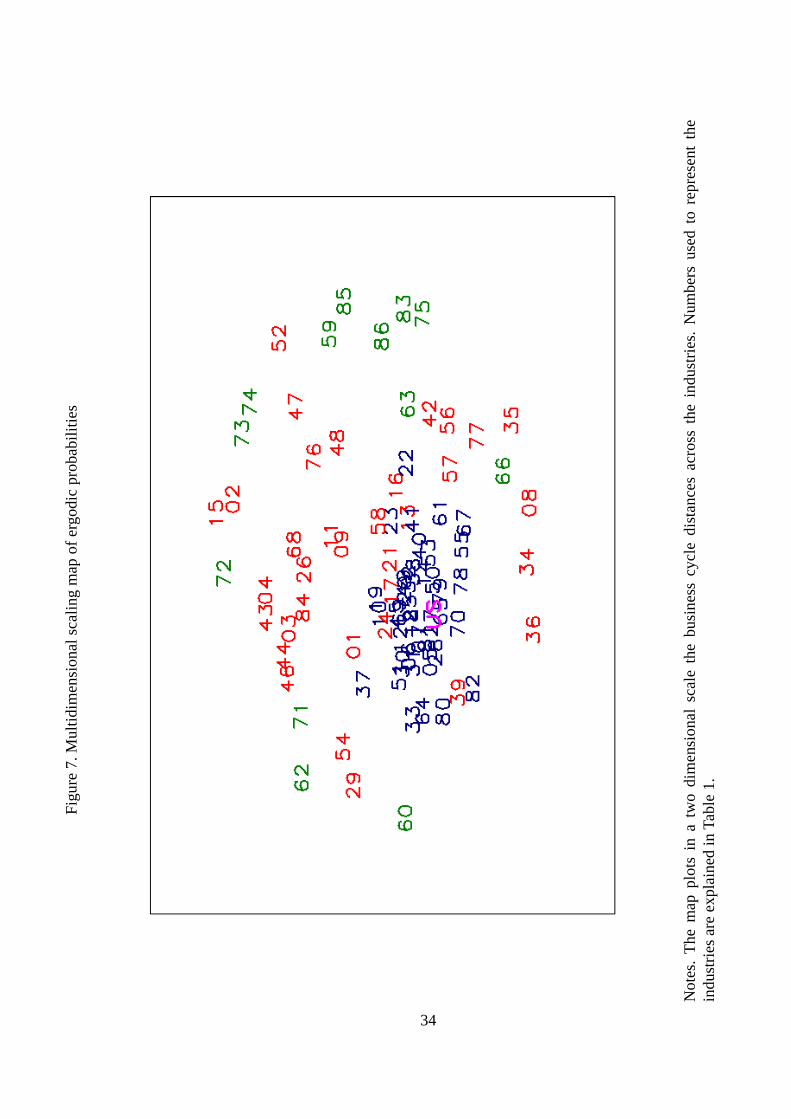
The multidimensional scaling map (see Appendix B) of business cycle similarities is reported

in Figure 7, whose plotted numbers refer to the industries listed in Table 1.4 Notably, the

industries grouped in the two/three di¤erent clusters of the dendogram belong to two/three

concentric circles, whose radius length re�ect the business cycle dissimilarities from the center

to the periphery. The US economy appears in the center or mass of the distribution of cyclical

similarities, re�ecting that some industries seem to stick together in the map and show business

cycle experiences that are similar to those of the nation. Although they are a relatively reduced

number of industries, they represent the 46:5% of the total US employment. However, the map

also shows an intermediary zone and a peripheral zone, indicating that other industries appear

away from the attractor and do not seem to be as closely related to the nation in business cycle

terms as the industries of the core. The intermediary and peripherial zone are composed by

industries representing the 20:6% and 32:9% per cent of total employment, respectively.

Let us have a deeper look at these business cycle a¢ liations. The core, in which the total

US employment is also included to facilitate comparison, is plotted in the center of the map

4 In these maps, the axes are meaningless and the orientation of the picture is arbitrary.

14

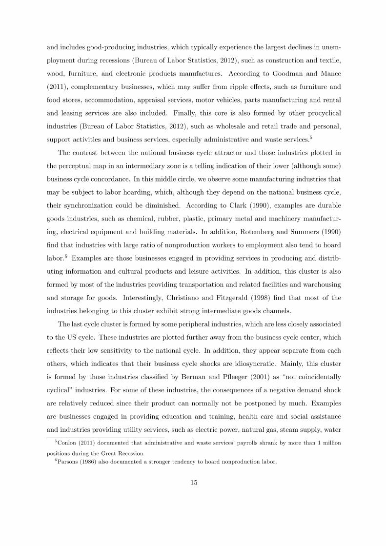
and includes good-producing industries, which typically experience the largest declines in unem-

ployment during recessions (Bureau of Labor Statistics, 2012), such as construction and textile,

wood, furniture, and electronic products manufactures. According to Goodman and Mance

(2011), complementary businesses, which may su¤er from ripple e¤ects, such as furniture and

food stores, accommodation, appraisal services, motor vehicles, parts manufacturing and rental

and leasing services are also included. Finally, this core is also formed by other procyclical

industries (Bureau of Labor Statistics, 2012), such as wholesale and retail trade and personal,

support activities and business services, especially administrative and waste services.5

The contrast between the national business cycle attractor and those industries plotted in

the perceptual map in an intermediary zone is a telling indication of their lower (although some)

business cycle concordance. In this middle circle, we observe some manufacturing industries that

may be subject to labor hoarding, which, although they depend on the national business cycle,

their synchronization could be diminished. According to Clark (1990), examples are durable

goods industries, such as chemical, rubber, plastic, primary metal and machinery manufactur-

ing, electrical equipment and building materials. In addition, Rotemberg and Summers (1990)

�nd that industries with large ratio of nonproduction workers to employment also tend to hoard

labor.6 Examples are those businesses engaged in providing services in producing and distrib-

uting information and cultural products and leisure activities. In addition, this cluster is also

formed by most of the industries providing transportation and related facilities and warehousing

and storage for goods. Interestingly, Christiano and Fitzgerald (1998) �nd that most of the

industries belonging to this cluster exhibit strong intermediate goods channels.

The last cycle cluster is formed by some peripheral industries, which are less closely associated

to the US cycle. These industries are plotted further away from the business cycle center, which

re�ects their low sensitivity to the national cycle. In addition, they appear separate from each

others, which indicates that their business cycle shocks are idiosyncratic. Mainly, this cluster

is formed by those industries classi�ed by Berman and P�eeger (2001) as �not coincidentally

cyclical�industries. For some of these industries, the consequences of a negative demand shock

are relatively reduced since their product can normally not be postponed by much. Examples

are businesses engaged in providing education and training, health care and social assistance

and industries providing utility services, such as electric power, natural gas, steam supply, water

5Conlon (2011) documented that administrative and waste services�payrolls shrank by more than 1 million

positions during the Great Recession.6Parsons (1986) also documented a stronger tendency to hoard nonproduction labor.

15

supply and sewage removal.7

In addition, this cluster includes sectors that highly depend on international shocks, such

as mineral extraction and their related supporting activities and gasoline stations, or on inter-

national competition, such as wholesale electronic markets.8 Belonging to this cluster, we also

�nd industries providing �nancial services, not because they were not cyclical, but because they

typically lead the national cycle.9 Finally, we �nd monetary authorities, federal state and local

government services. These industries provide necessities or public goods and demand for these

goods remain relatively strong throughout lows of the economy.

3.4 Evolution of linkages

How have the industrial business cycle linkages evolved over time? Traditionally, the literature

would address this question by dividing the full sample into several sub-periods. The problem

of this approach is that it would provide pictures of the cycle linkages that rely on speci�c date

breaks, whose location is sometimes controversial. To overcome this drawback, the pairwise

probabilities of cycle dependence p (vab;t = i) for all industries a, b, are collected for all periods

t. Now, kernel density estimates, multimodality tests and multidimensional scaling maps can

be calculated for each month of the sample. Accordingly, the pictures provided above become

animated videos that allows one to easily identify which industries manifested the �rst signs of

phase changes and to examine how the interconnections across industries propagate the business

cycle shocks across industries.10

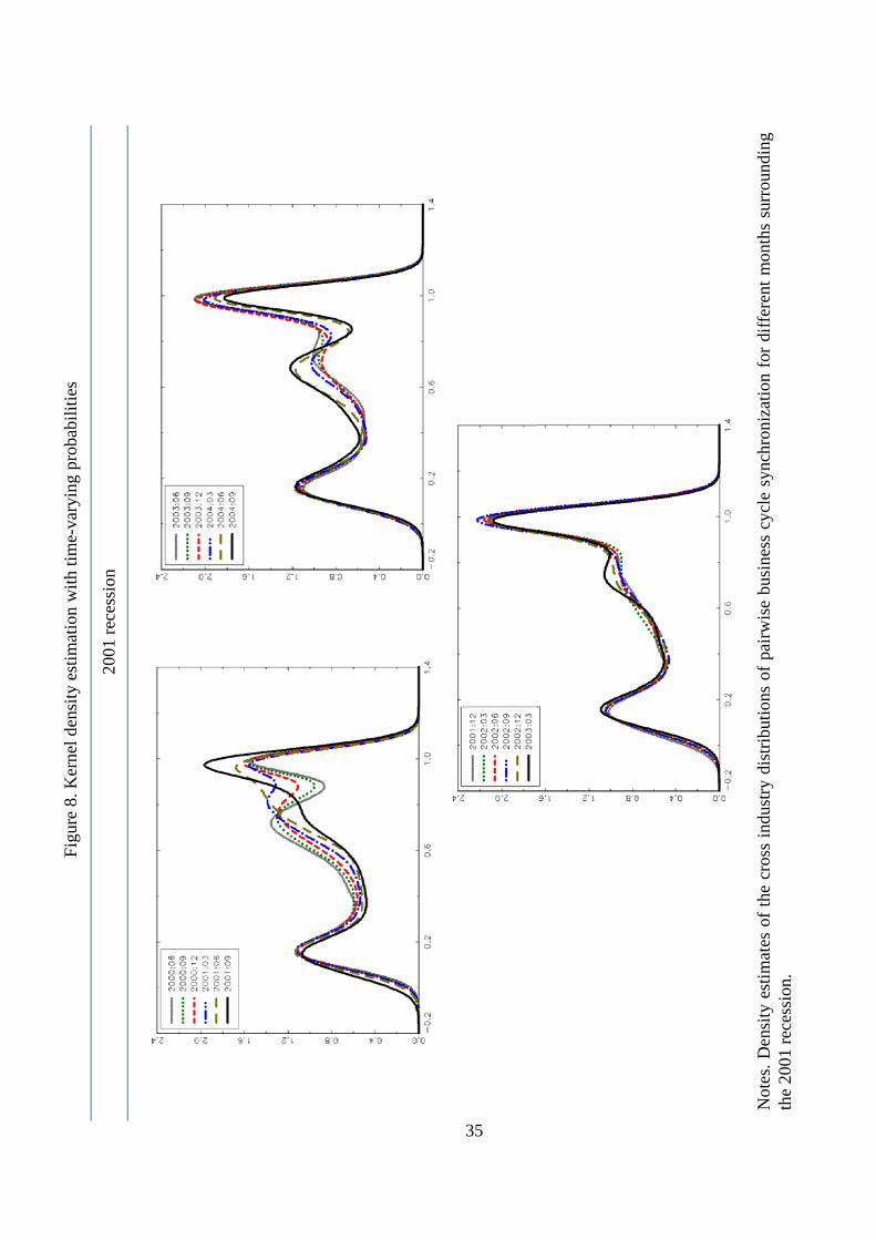
To examine the intra-distribution evolution of business cycle proximities, Figure 8 and Figure

9 plot the overlaid families of empirical kernel distributions across several months around the

2001 and 2008 recessions, respectively. In interpreting these charts, it is worth emphasizing that

the horizontal axis measures pairwise business cycle dissimilarities. Therefore, each right-hand

horizontal movement represents absolute losses in pairwise synchronization among industries.

Figure 8 shows that some months before the 2001 recession, the densities exhibited a trimodal

7Goodman (2001) �nds out that private education and health services are countercyclical. In fact, employment

has decreased in only 1 of the 12 NBER recessions that have occurred since 1945 (Bureau of Labor Statistics,

2012).8Groshen and Potter (2003) �nd that oil and gas extraction �rms are countercyclical.9Christiano and Fitzgerald (1998) �nd that the business cycle components of �nance, insurance, and real estate

industry exhibit low contemporaneous comovement with aggregate employment. Goodman and Mance (2011)

show that employment in �nancial activities peaked one year before the o¢ cial start of the Great Recession.10 The full animated graphs of this paper can be found at http://www.um.es/econometria/Maximo.

16

distribution of business cycle distances, agreeing with the pattern obtained in the multidimen-

sional scaling analysis. That is, we �nd a core composed by industries highly synchronized with

each other (left-hand mode), a group of moderately synchronized industries (middle mode) and

some idiosyncratic industries that follow independent cyclical patterns (right-hand side mode).

However, as the economy approached to the recession, the distribution tended to reshape to

bimodal. This happened because industries did not fall into the recession simultaneously but

sequentially, as noticed in Figure 3. The �rst industries falling to the recession were those of the

core while the industries that belonged to the middle mass remained in expansion. This reduced

the synchronization and pushed to the right-hand side part the middle mass of the distribution.

During the recession, more industries changed the phase cycle, which implied that a third

mode appeared again in the middle of the distribution. However, when the trough takes place,

the cyclical position was reversed back. The core changed the phase cycle �rst, which accentuated

the business cycle discrepances with the middle mass, which shifted again to the right. Therefore,

the distribution was reshaped to bimodal as it did in the peak. Finally, the middle mode

appeared again when more industries initiated the recovery phase following the core.

A similar but more accentuated pattern occurred during the 2008 recession. Figure 9 shows

that before the recession started the distribution seemed to be characterized by three modes.

When the peak occurred the distribution became bimodal, since industries fell in recession in a

sequential way providing evidence of a cascade e¤ect. Once the economy was in recession the

trimodal pattern in the distribution was recovered until the peak, where only the industries of

the core initiated the recovery and the distribution became bimodal again. The cycle ended

when the economy returned to the stable expansionary phase, and the distribution presented

three modes, which remained until the next turning point.

In sum, we �nd that the propagation of micro-level shocks to national shocks is enhanced

when the mass shifts that characterizes the turning points occur. A formal statistical test of this

pattern is provided by applying the modality tests in the density distributions of business cycle

similarities from 1991:01 to 2013:05. According to the plots of the kernel densities, the nulls of

unimodality (not shown to save space) were clearly rejected for all months since the p-values

were always pretty close to zero. Figure 10 plots the p-values of the null of two versus three

modes. To facilitate the analysis, the �gure included shaded areas that refer to the NBER-

referenced recessions and a dashed line that refers to the 0:05 signi�cance level. The �gure

shows that bimodality is rejected during the national expansions and recessions while it cannot

17

be rejected at any reasonable signi�cance level when the turning points arrive.11 Notably, the

lagged business cycle behavior that characterized employment implies that bimodality appears

with some lags with respect to the NBER turning points. Therefore, the Silverman test con�rms

the mass shift in turning points documented above. In other words, the time-varying p-values

reaching the 0:05 threshold could be interpreted as indicators of national turning points on

(employment) cycles.

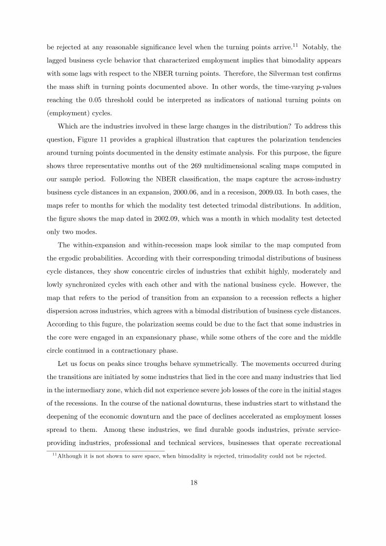
Which are the industries involved in these large changes in the distribution? To address this

question, Figure 11 provides a graphical illustration that captures the polarization tendencies

around turning points documented in the density estimate analysis. For this purpose, the �gure

shows three representative months out of the 269 multidimensional scaling maps computed in

our sample period. Following the NBER classi�cation, the maps capture the across-industry

business cycle distances in an expansion, 2000:06, and in a recesison, 2009:03. In both cases, the

maps refer to months for which the modality test detected trimodal distributions. In addition,

the �gure shows the map dated in 2002:09, which was a month in which modality test detected

only two modes.

The within-expansion and within-recession maps look similar to the map computed from

the ergodic probabilities. According with their corresponding trimodal distributions of business

cycle distances, they show concentric circles of industries that exhibit highly, moderately and

lowly synchronized cycles with each other and with the national business cycle. However, the

map that refers to the period of transition from an expansion to a recession re�ects a higher

dispersion across industries, which agrees with a bimodal distribution of business cycle distances.

According to this fugure, the polarization seems could be due to the fact that some industries in

the core were engaged in an expansionary phase, while some others of the core and the middle

circle continued in a contractionary phase.

Let us focus on peaks since troughs behave symmetrically. The movements occurred during

the transitions are initiated by some industries that lied in the core and many industries that lied

in the intermediary zone, which did not experience severe job losses of the core in the initial stages

of the recessions. In the course of the national downturns, these industries start to withstand the

deepening of the economic downturn and the pace of declines accelerated as employment losses

spread to them. Among these industries, we �nd durable goods industries, private service-

providing industries, professional and technical services, businesses that operate recreational

11Although it is not shown to save space, when bimodality is rejected, trimodality could not be rejected.

18

interests, and industries providing transportation, warehousing and storage for goods.

These industries fall when there is no way back in the national recession, which become

a clear sign of a phase shift. We postulate that this salient characteristic of peaks could be

caused by, at least, one of the following determinants. First, since investments in durable goods

can usually be postponed, buyers can bene�t from waiting to receive more information about

how the economy develops. Therefore, the contagion only appears when the recession becomes

more evident. Second, although labor hoarding guarantees employee talent will be available, the

practice implies high risks as it reduces companies�pro�tability during the di¢ cult times. When

the bad times are prolonged, their negative consequences become unavoidable. Third, some of

the output of the consumption good sector, which lay in the core, is also used as intermediate

goods in the production of durable goods, such as machinery and equipment, which lay in the

middle mass. During the recession, the durable goods industries are seriously exposed to ripple

e¤ects, which come from the core with some lags.

4 Concluding remarks

This paper is part of a growing empirical literature that analyze the sources of interindustry co-

movements. It di¤ers from this literature in several of the following aspects. Firstly, the approach

is in the mould of �measurement without theory�. We are asking whether the industry-level

business cycles cohere on employment data not only with the national business cycle but also

with each other. Secondly, the �lter used to compute the business cycle inferences is an exten-

sion of the Markov-switching �lter that allows for time-varying business cycle interdependence.

Thirdly, nonparametric density estimation techniques are applied to assess the degree of pop-

ulation heterogeneity and to examine the changes on the business cycle distribution. Finally,

heuristic techniques of classical multidimensional scaling and clustering are used to understand

the industry movements going in and out of recessions, which helps us to identify changes in

cyclical a¢ liations.

Our main results are the following. First, there is a large heterogeneity in the distribution

of business cycle similarities, implying the existence of population groups that follow distinct

distributional dynamics. Second, there is not a monotone movement towards the emergence of

an increasingly cohesive national business cycle core. The position of the lower mode, which

comprises extremely synchronized industries, and the cluster at the high end of the distribu-

19

tion, which represents the industries with idiosyncratic cycles, are relatively stable over time.

However, the position of a third middle mode prevailing once the economy is in expansionary

or recessionary phases jumps up substantially during the period of transition from one phase to

another, switching from pairwise business cycle distances of just over 0:5 to almost one. There-

fore, the proposed framework is able to provide assessments about when a national turning point

takes place and how the business cycle shocks propagate across industries.

The model used in this paper provides a solid foundation for starting a line of research that

seeks to explain the determinants of the business cycle a¢ liations across industries. Various

factors have been put forward in the literature that may a¤ect business cycle synchronization,

ranging from the proportion of �xed and variable costs, industry concentration, product di¤er-

entiation and dependence on external �nance. However, the modi�cations of the model used in

the paper to capture the a¢ liations changes would be substantial and this task is left to further

research.

20

Appendix AThis appendix describes the estimation of the parameters in vector � and the inference ones�ab;T , which is performed through a multi-move Gibbs-sampling procedure. Their distributions

can be approximated by the empirical distributions of simulated values, by iterating the following

steps.

STEP 1. The Gibbs sampler is started with arbitrary starting values for the parameters of

the model, �0, which are used to generate es�1ab;T jeyab;T ; �0. For this purpose, we run the Markov-switching �lter described in Section 2 and obtain the �ltered probabilities p(s�ab;tjeyab;t; �0). Todraw the state variables, we employ the following result

p�es�ab;T jeyab;T ; �0� = p �s�ab;T jeyab;T ; �0� T�1Y

t=1

p(s�ab;tjs�ab;t+1; eyab;t; �0): (A1)

The last iteration of the Markov-switching �lter provides us with p�s�ab;T jeyab;T ; �0�, from which

is s�ab;T generated. To generate s�ab;t, with t = 1; :::; T � 1, we use

p(s�ab;tjs�ab;t+1; eyab;t; �0) = p(s�ab;t+1js�ab;t) / p(s�ab;tjeyab;t; �0); (A2)

where p(s�ab;tjs�ab;t+1) refers to the transition probabilities, which are included in �0. Using this

expression, it is straightforward to generate s�ab;t by computing the probability of state i from

p(s�ab;t = ijs�ab;t+1; eyab;t; �0) = p(s�ab;t+1js�ab;t = i)p(s�ab;t = ijeyab;t; �0)Pj 6=ip(s�ab;t+1js�ab;t = j)p(s�ab;t = jjeyab;t; �0) : (A3)

Using random numbers from a uniform distribution between 0 and 1, s�1ab;t is set to a par-

ticular state i by comparing the probability of this state with the random numbers. Follow-

ing a similar reasoning, one can also generate es1k;T = s1k;1; :::; s1k;T , ev1ab;T = v1ab;1; :::; v

1ab;T ande&1ab;T = &1ab;1; :::; &1ab;T , for any industry k and any pair a and b at any time t = 1; :::; T .

STEP 2. The generated state variables are used to draw the transition probabilities pkij , pabij

and qabij . Since these parameters are drawn in a similar way, we focus only on pkij to save space.

Conditional on esk;T , the transition probabilities are independent on the data set eyab;T and themodel�s other parameters. Given es1k;T , let nkij , i; j = 0; 1, be the total number of transitions fromsate i to state j in industry k. By taking the beta family of distributions as conjugate priors

pkii~beta(ukii; u

kij); (A4)

21

where ukii and ukij are known parameters of the priors, it can be shown that the posterior

distributions of pkii are given by

pkiijesk;T ; eyab;T ~beta(ukii + nkii; ukij + nkij); (A5)

from which pk1ii are drawn. In particular, we set uk00 = 8, u

k01 = 2, u

k11 = 0 and u

k10 = 1 for all k.

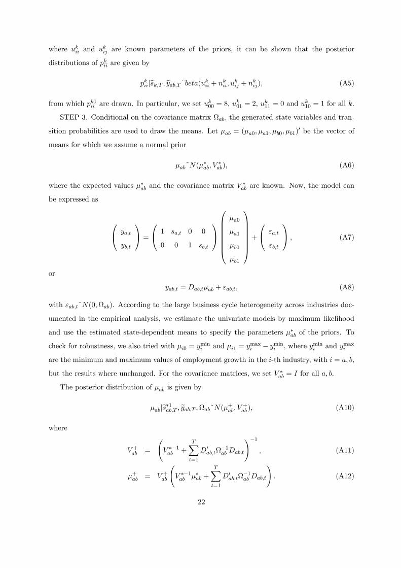
STEP 3. Conditional on the covariance matrix ab, the generated state variables and tran-

sition probabilities are used to draw the means. Let �ab = (�a0; �a1; �b0; �b1)0 be the vector of

means for which we assume a normal prior

�ab~N(��ab; V

�ab); (A6)

where the expected values ��ab and the covariance matrix V�ab are known. Now, the model can

be expressed as

0@ ya;t

yb;t

1A =

0@ 1

0

sa;t

0

0

1

0

sb;t

1A0BBBBBB@�a0

�a1

�b0

�b1

1CCCCCCA+0@ "a;t

"b;t

1A ; (A7)

or

yab;t = Dab;t�ab + "ab;t; (A8)

with "ab;t~N(0;ab). According to the large business cycle heterogeneity across industries doc-

umented in the empirical analysis, we estimate the univariate models by maximum likelihood

and use the estimated state-dependent means to specify the parameters ��ab of the priors. To

check for robustness, we also tried with �i0 = ymini and �i1 = y

maxi � ymini , where ymini and ymaxi

are the minimum and maximum values of employment growth in the i-th industry, with i = a; b,

but the results where unchanged. For the covariance matrices, we set V �ab = I for all a; b.

The posterior distribution of �ab is given by

�abjes�1ab;T ; eyab;T ;ab~N(�+ab; V +ab ); (A10)

where

V +ab =

V ��1ab +

TXt=1

D0ab;t�1ab Dab;t

!�1; (A11)

�+ab = V +ab

V ��1ab ��ab +

TXt=1

D0ab;t�1ab Dab;t

!: (A12)

22

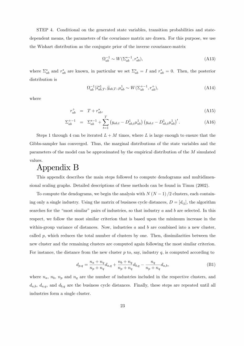
STEP 4. Conditional on the generated state variables, transition probabilities and state-

dependent means, the parameters of the covariance matrix are drawn. For this purpose, we use

the Wishart distribution as the conjugate prior of the inverse covariance-matrix

�1ab �W (��1ab ; r

�ab); (A13)

where ��ab and r�ab are known, in particular we set �

�ab = I and r�ab = 0. Then, the posterior

distribution is

�1ab jes�1ab;T ; eyab;T ; �1ab �W (�+�1ab ; r+ab); (A14)

where

r+ab = T + r�ab; (A15)

�+�1ab = ��1ab +

TXt=1

�yab;t �D1ab;t�1ab

� �yab;t �D1ab;t�1ab

�0: (A16)

Steps 1 through 4 can be iterated L+M times, where L is large enough to ensure that the

Gibbs-sampler has converged. Thus, the marginal distributions of the state variables and the

parameters of the model can be approximated by the empirical distribution of the M simulated

values.

Appendix BThis appendix describes the main steps followed to compute dendograms and multidimen-

sional scaling graphs. Detailed descriptions of these methods can be found in Timm (2002).

To compute the dendograms, we begin the analysis with N (N � 1) =2 clusters, each contain-

ing only a single industry. Using the matrix of business cycle distances, D = [dij ], the algorithm

searches for the �most similar�pairs of industries, so that industry a and b are selected. In this

respect, we follow the most similar criterion that is based upon the minimum increase in the

within-group variance of distances. Now, industries a and b are combined into a new cluster,

called p, which reduces the total number of clusters by one. Then, dissimilarities between the

new cluster and the remaining clusters are computed again following the most similar criterion.

For instance, the distance from the new cluster p to, say, industry q, is computed according to

dp;q =na + nqnp + nq

da;q +nb + nqnp + nq

db;q �nq

np + nqda;b; (B1)

where na, nb, np and nq are the number of industries included in the respective clusters, and

da;b, da;q, and db;q are the business cycle distances. Finally, these steps are repeated until all

industries form a single cluster.

23

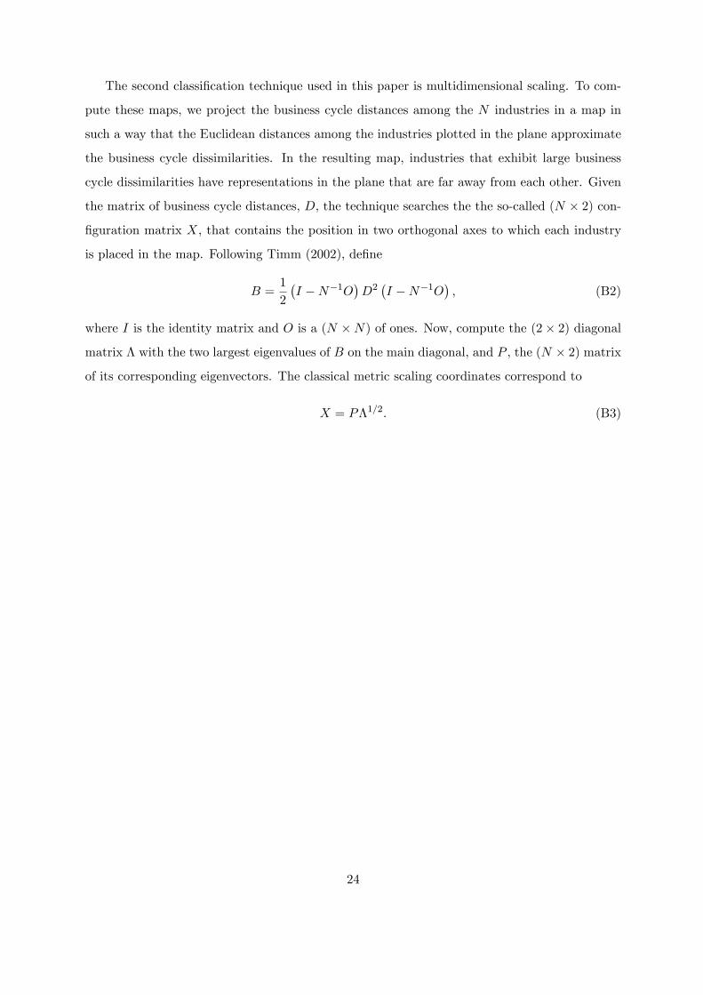
The second classi�cation technique used in this paper is multidimensional scaling. To com-

pute these maps, we project the business cycle distances among the N industries in a map in

such a way that the Euclidean distances among the industries plotted in the plane approximate

the business cycle dissimilarities. In the resulting map, industries that exhibit large business

cycle dissimilarities have representations in the plane that are far away from each other. Given

the matrix of business cycle distances, D, the technique searches the the so-called (N � 2) con-

�guration matrix X, that contains the position in two orthogonal axes to which each industry

is placed in the map. Following Timm (2002), de�ne

B =1

2

�I �N�1O

�D2�I �N�1O

�; (B2)

where I is the identity matrix and O is a (N �N) of ones. Now, compute the (2� 2) diagonal

matrix � with the two largest eigenvalues of B on the main diagonal, and P , the (N � 2) matrix

of its corresponding eigenvectors. The classical metric scaling coordinates correspond to

X = P�1=2: (B3)

24

References

[1] Acemoglu, D., Carvalho, V., Ozdaglar, A., and Tahbaz-Salehi, A. 2012 . The network origins

of aggregate �uctuations. Econometrica 80: 1977-2016.

[2] Bengoechea, P., Camacho, M., and Perez Quiros, G. 2006. A useful tool for forecasting the

Euro-area business cycle phases International Journal of Forecasting 22: 735-749.

[3] Berman, J. and P�eeger, J. 1992. Which industries are sensitive to business cycles? Monthly

Labor Review February: 19-25.

[4] Bureau of Labor Statistics. 2012. The recession of 2007-2009. BLS Spotlight on Statistics,

February.

[5] Camacho, M., and Perez Quiros, G. 2006. A new framework to analyze business cycle

synchronization. In: Milas, C., Rothman, P., and van Dijk, D. Nonlinear Time Series

Analysis of Business Cycles. Elsevier�s Contributions to Economic Analysis series. Chapter

5 (pp. 133-149). Elsevier, Amsterdam.

[6] Carlino, G., de Fina, H. 2004. How strong is co-movement in employment over the business

cycle? Evidence from state/industry data. Journal of Urban Economics 55: 298-315.

[7] Christiano, L., and Fitzgerald, T. 1998. The business cycle: it�s still a puzzle. Economic

Perspectives, Fourth Quarter: 56-83.

[8] Clark, S. 1973. Labor hoarding in durable goods industries. American Economic Review

63: 811-824.

[9] Conlon. F. 2011. Professional and business services: employment trends in the 2007-09

recession. Monthly Labor Review April: 34-39.

[10] Filardo, A. 1997. Cyclical implications of the declining manufacturing employment share.

Federal Reserve Bank of Kansas City Economic Review II: 63-87.

[11] Foerster, A., Sarte, P., and Watson, M. 2011. Sectorial versus aggregate shocks: a structural

factor analysis of industrial production. Journal of Political Economy 119: 1-38.

[12] Groshen, E., and Potter, S. 2003. Has structural change contributed to a jobless recovery?

Current Issues in Economics and Finance 9 (August).

25

[13] Gavaix, X. 2011. The granular origins of aggregate �uctuations. Econometrica 79: 733-772.

[14] Goodman, W. 2001. Employment in services industries a¤ected by recessions and expan-

sions. Monthly Labor Review October: 3-11.

[15] Goodman, W., and Mance, S. 2011. Employment loss and the 2007-09 recession: an

overview. Monthly Labor Review April: 3-12.

[16] Hamilton, J. 1989. A new approach to the economic analysis of nonstationary time series

and the business cycles. Econometrica 57: 357-384.

[17] Leiva Leon, D. 2014. A New Approach to Infer Changes in the Synchronization of Business

Cycle Phases. Working Paper, Bank of Canada.

[18] Malmendier, U., and Nagel, S. 2011. Depression babies: Do macroeconomic experiences

a¤ect risk taking? The Quarterly Journal of Economics 126: 373-416.

[19] Owan, M., Piger, J., and Wall, H. 2005. Business cycle phases in the U.S. states. The Review

of Economics and Statistics 87: 604-616.

[20] Owan, M., Piger, J., Wall, H., and Wheeler, Ch. 2008. The economic performance of cities:

A Markov-switching approach. Journal of Urban Economics 64: 538-550.

[21] Parsons O. 1986. The employment relationship: Job attachment, work e¤ort and the nature

of contracts. In Handbook of Labor Economics. Ashenfelter O, Layard R (eds.), Elsevier:

New York.

[22] Rotemberg J, and Summers L. 1990. In�exible Prices and Procyclical productivity. Quar-

terly Journal of Economics 105: 851-874.

[23] Silverman, B. 1981. Using kernel density estimates to investigate multimodality. Journal of

the Royal Statistical Society, Series B 43: 97-99.

[24] Tan, H., and Mathews, J. 2010. Identi�cation and analysis of industry cycles. Journal of

Business Research 63: 454-462.

[25] Timm, N. 2002. Applied multivariate analysis. Springer texts in Statistics.

[26] Urquhart, M. 1981. The services industry: Is it recession-proof? Monthly Labor Review

October: 12-18.

26

27

Table 1. Properties of the sectorial business cycles

Industry, 3 digits Averaged growth rates

Total Expansion Recession Forestry (1) -2.17 -1.52 -7.60 Oil and Gas Extraction (2) 0.15 -0.38 4.58 Mining, except Oil and Gas (3) -1.26 -1.23 -1.53 Support Activities for Mining (4) 4.03 3.74 6.39 Construction of Buildings (5) -0.35 0.62 -8.38 Heavy and Civil Engineering Construction (6) 0.47 1.02 -4.10 Specialty Trade Contractors (7) 0.93 1.79 -6.18 Food Manufacturing (8) -0.10 -0.05 -0.44 Textile Mills (9) -6.08 -5.30 -12.51 Textile Product Mills (10) -3.01 -2.40 -8.02 Apparel Manufacturing (11) -7.66 -7.26 -10.96 Wood Product Manufacturing (12) -1.83 -0.58 -12.20 Paper Manufacturing (13) -2.35 -2.10 -4.37 Printing and Related Support Activities (14) -2.45 -2.04 -5.79 Petroleum and Coal Products Manufacturing (15) -1.27 -1.49 0.51 Chemical Manufacturing (16) -1.20 -1.05 -2.48 Plastics and Rubber Products Manufacturing (17) -0.96 -0.29 -6.48 Nonmetallic Mineral Product Manufacturing (18) -1.55 -0.84 -7.42 Primary Metal Manufacturing (19) -2.23 -1.59 -7.56 Fabricated Metal Product Manufacturing (20) -0.43 0.17 -5.35 Machinery Manufacturing (21) -0.96 -0.54 -4.42 Computer and Electronic Product Manufacturing (22) -2.35 -2.11 -4.34 Electrical Equipment, Appliance, and Component Manufacturing (23)

-2.30 -1.96 -5.06

Transportation Equipment Manufacturing (24) -1.52 -0.71 -8.20 Furniture and Related Product Manufacturing (25) -2.21 -1.18 -10.71 Miscellaneous Manufacturing (26) -1.98 -1.90 -2.64 Merchant Wholesalers, Durable Goods (27) 0.07 0.54 -3.78 Merchant Wholesalers, Nondurable Goods (28) 0.21 0.43 -1.61 Wholesale Electronic Markets and Agents and Brokers (29) 2.28 2.63 -0.55 Motor Vehicle and Parts Dealers (30) 0.76 1.41 -4.58 Furniture and Home Furnishings Stores (31) 0.27 1.19 -7.39 Electronics and Appliance Stores (32) 0.63 1.18 -3.94 Building Material and Garden Equipment and Supplies Dealers (33)

1.29 1.88 -3.61

Food and Beverage Stores (34) 0.17 0.23 -0.36 Health and Personal Care Stores (35) 1.13 1.20 0.56 Gasoline Stations (36) -0.31 -0.12 -1.95 Clothing and Clothing Accessories Stores (37) 0.42 0.81 -2.80 Sporting Goods, Hobby, Book, and Music Stores (38) 1.05 1.29 -0.91 General Merchandise Stores (39) 0.97 1.14 -0.40 Miscellaneous Store Retailers (40) 0.46 0.90 -3.16 Nonstore Retailers (41) 0.31 0.61 -2.14 Air Transportation (42) -0.62 -0.55 -1.16 Rail Transportation (43) -0.68 -0.47 -2.43 Water Transportation(44) 0.55 0.73 -0.89 Truck Transportation (45) 0.94 1.52 -3.82 Transit and Ground Passenger Transportation (46) 2.34 2.42 1.68 Pipeline Transportation (47) -1.27 -1.70 2.31 Scenic and Sightseeing Transportation (48) 2.59 2.79 1.00 Support Activities for Transportation (49) 2.18 2.46 -0.12 Couriers and Messengers (50) 1.69 2.19 -2.44

28

Warehousing and Storage (51) 2.41 2.80 -0.75 Utilities (52) -1.26 -1.48 0.55 Publishing Industries, except Internet (53) -0.71 -0.40 -3.23 Motion Picture and Sound Recording Industries (54) 1.93 2.47 -2.50 Broadcasting, except Internet (55) 0.05 0.27 -1.73 Telecommunications (56) -0.59 -0.53 -1.07 Data Processing, Hosting, and Related Services (57) 0.85 1.24 -2.37 Other Information Services (58) 5.54 6.11 0.84 Monetary Authorities - Central Bank (59) -1.47 -1.73 0.76 Credit Intermediation and Related Activities (60) 0.34 0.69 -2.56 Securities, Commodity Contracts, and Other Financial Investments and Related Activities (61)

2.73 3.04 0.22

Insurance Carriers and Related Activities (62) 0.69 0.71 0.47 Funds, Trusts, and Other Financial Vehicles (63) 2.24 2.22 2.33 Real Estate (64) 1.14 1.35 -0.59 Rental and Leasing Services (65) 0.10 0.59 -3.95 Lessors of Nonfinancial Intangible Assets, except Copyrighted Works (66)

2.58 2.94 -0.43

Professional, Scientific, and Technical Services (67) 2.60 2.83 0.66 Management of Companies and Enterprises (68) 0.89 0.98 0.11 Administrative and Support Services (69) 2.69 3.76 -6.16 Waste Management and Remediation Services (70) 2.24 2.47 0.32 Educational Services (71) 3.14 3.06 3.77 Ambulatory Health Care Services (72) 3.70 3.74 3.42 Hospitals (73) 1.42 1.30 2.40 Nursing and Residential Care Facilities (74) 2.47 2.41 2.97 Social Assistance (75) 4.16 4.22 3.67 Performing Arts, Spectator Sports, and Related Industries (76) 1.94 2.20 -0.25 Museums, Historical Sites, and Similar Institutions (77) 3.20 3.39 1.62 Amusement, Gambling, and Recreation Industries (78) 2.73 3.03 0.20 Accommodation (79) 0.57 0.89 -2.07 Food Services and Drinking Places (80) 1.97 2.19 0.14 Repair and Maintenance (81) 0.80 1.20 -2.45 Personal and Laundry Services (82) 0.76 0.85 0.03 Religious, Grantmaking, Civic, Professional, and Similar Organizations (83)

1.46 1.45 1.53

Federal (84) -0.55 -0.58 -0.30 State Government (85) 0.72 0.62 1.55 Local Government (86) 1.14 1.09 1.54 USA 0.94 1.20 -1.23

Notes. Industries by NAICS Code. Numbers and acronyms with which they appear in multidimensional scaling maps are in brackets. Last three columns refer to the (total, within the NBER expansions and within the NBER recessions) average growth rate of employment.

Table 2. Bootstrap multimodality tests

N. modes under null

Critical bandwith

p-value

1 0.141 0.00

2 0.031 0.27

3 0.028 0.12

4 0.021 0.26

Notes. Each row shows the number of modes under the null, the critical bandwidth and the corresponding p-value of the Silverman’s test.

Fig

ure

1. U

S e

mpl

oym

ent

4 ‐202 ‐6‐4 1991.01

1995.06

1999.11

2004.04

2008.09

2013.02

Not

es. T

he f

igur

e pl

ots

annu

al g

row

th r

ates

. Sha

ded

area

s re

fer

to N

BE

R r

eces

sion

.

Fig

ure

2. K

erne

l dis

trib

utio

n ov

er th

e cy

cle

2

.12

.16

.20

y

Exp

ansi

on

9

.00

.04

.08

Density

Rec

essi

on

Not

es.

The

figu

repl

ots

the

kern

eldi

stri

buti

onof

y-o-

yem

ploy

men

tgr

owth

acro

ssin

dust

ries

.E

xpan

sion

san

dre

cess

ions

are

obta

ined

from

the

NB

ER

busi

ness

cycl

eda

tes.

-16

-14

-12

-10

-8-6

-4-2

02

46

81

0

Fig

ure

3. U

niva

riat

eM

arko

v-sw

itch

ing

anal

ysis

2001

rec

essi

on

1999

Q4

2000

Q1

2000

Q2

2000

Q3

2000

Q4

1999

Q4

2000

Q1

2

000Q

2

20

00Q

3

2

000Q

4

2001

Q1

200

1Q2

2001

Q3

2001

Q4

20

02Q

1

2002

Q2

200

2Q3

2002

Q4

200

3Q1

200

3Q2

30

0.0

0.2

0

.4

0.6

0

.8

1.0

Not

es.

The

figu

repl

ots

the

chor

ople

thm

apof

indu

stri

esfo

rdi

ffer

ent

quar

ters

surr

ound

ing

the

2001

rece

ssio

n(b

old

red

lett

ers)

.E

ach

char

tco

rres

pond

sto

one

quar

ter,

the

part

itio

nsof

each

char

tre

pres

ent

the

U.S

.in

dust

ries

and

thei

rsi

zere

pres

ents

thei

rsh

are

ofth

ena

tion

alem

ploy

men

t.T

heda

rker

isan

indu

stry

the

high

eris

the

prob

abil

ity

ofre

cess

ion

for

that

indu

stry

duri

ngth

atqu

arte

r.

Fig

ure

4. U

niva

riat

eM

arko

v-sw

itch

ing

anal

ysis

2007

Q2

2007

Q3

2007

Q4

2008

Q1

2008

Q2

2008

rec

essi

on

2007

Q2

200

7Q3

200

7Q4

200

8Q1

2008

Q2

2008

Q3

200

8Q4

200

9Q1

200

9Q2

20

09Q

3

2009

Q4

201

0Q1

201

0Q2

2010

Q3

201

0Q4

31

0.0

0.2

0

.4

0.6

0

.8

1.0

Not

es.

The

figu

repl

ots

the

chor

ople

thm

apof

indu

stri

esfo

rdi

ffer

ent

quar

ters

surr

ound

ing

the

2008

rece

ssio

n(b

old

red

lett

ers)

.E

ach

char

tco

rres

pond

sto

one

quar

ter,

the

part

itio

nsof

each

char

tre

pres

ent

the

U.S

.in

dust

ries

and

thei

rsi

zere

pres

ents

thei

rsh

are

ofth

ena

tion

alem

ploy

men

t.T

heda

rker

isan

indu

stry

the

high

eris

the

prob

abil

ity

ofre

cess

ion

for

that

indu

stry

duri

ngth

atqu

arte

r.

Fig

ure

5. K

erne

l den

sity

est

imat

ion

from

erg

odic

prob

abil

itie

s

32

Not

es.D

ensi

tyes

tim

ates

ofth

ecr

oss

indu

stry

dist

ribu

tion

sof

pair

wis

ebu

sine

sscy

cle

sync

hron

izat

ion

usin

ger

godi

cpr

obab

ilit

ies.

Fig

ure

6. C

lust

er a

naly

sis

wit

h er

godi

cpr

obab

ilit

ies

2

1.5

0.51

1453

4578

6 7

5570

8119

2750

6920

7938

5167

US82

2223

4132

6140

49 5

2810

6465

1218

3325

3037

3180

117

26 9

1311

1624

343

2168

2 4

1547

52 8

3577

2954

3436

3984

4476

4642

5657

5848

5985

7375

8660

6263

6671

8372

740

33

Not

es.

The

dend

ogra

m’s

heig

hts

repr

esen

tth

ele

vel

ofdi

ssim

ilar

ity

atw

hich

obse

rvat

ions

orcl

uste

rsar

em

erge

d.N

umbe

rsus

edto

repr

esen

tthe

indu

stri

esar

eex

plai

ned

inTa

ble

1.

Fig

ure

7. M

ulti

dim

ensi

onal

sca

ling

map

of

ergo

dic

prob

abil

itie

s

34

Not

es.

The

map

plot

sin

atw

odi

men

sion

alsc

ale

the

busi

ness

cycl

edi

stan

ces

acro

ssth

ein

dust

ries

.N

umbe

rsus

edto

repr

esen

tth

ein

dust

ries

are

expl

aine

din

Tabl

e1.

Fig

ure

8. K

erne

l den

sity

est

imat

ion

wit

h ti

me-

vary

ing

prob

abil

itie

s

2001

rec

essi

on

35

Not

es.

Den

sity

esti

mat

esof

the

cros

sin

dust

rydi

stri

buti

ons

ofpa

irw

ise

busi

ness

cycl

esy

nchr

oniz

atio

nfo

rdi

ffer

ent

mon

ths

surr

ound

ing

the

2001

rece

ssio

n.

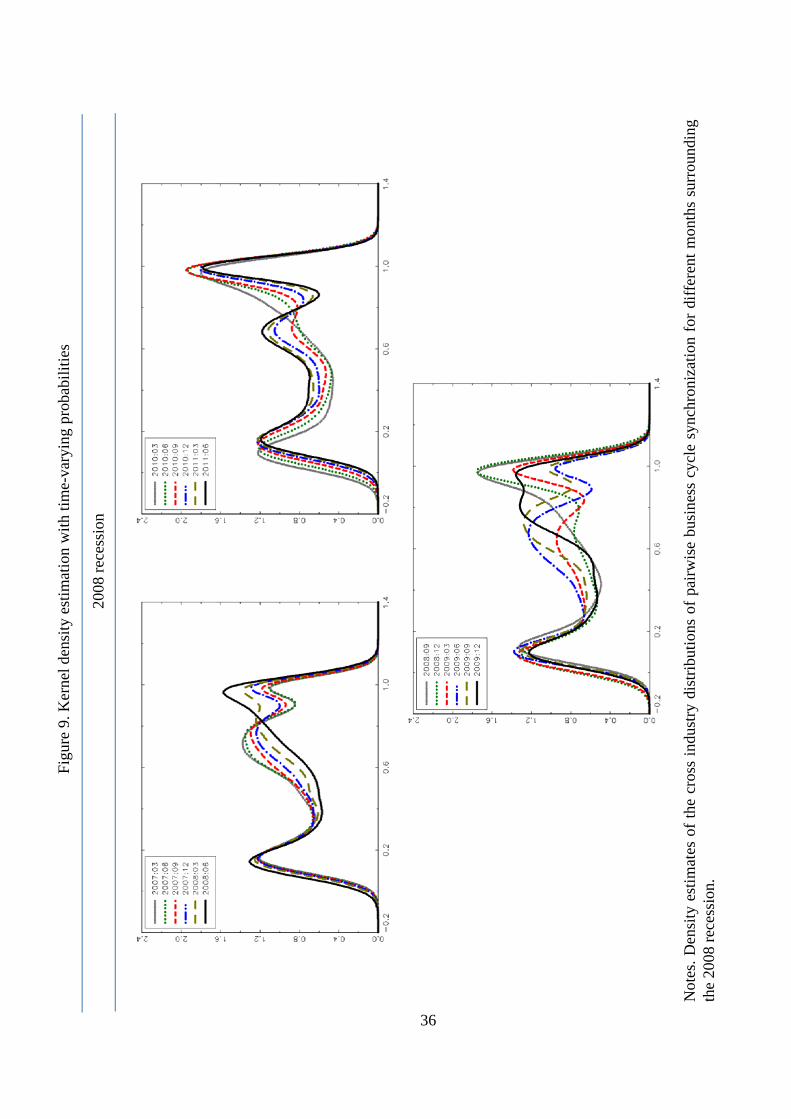
Fig

ure

9. K

erne

l den

sity

est

imat

ion

wit

h ti

me-

vary

ing

prob

abil

itie

s

2008

rec

essi

on

36

Not

es.

Den

sity

esti

mat

esof

the

cros

sin

dust

rydi

stri

buti

ons

ofpa

irw

ise

busi

ness

cycl

esy

nchr

oniz

atio

nfo

rdi

ffer

ent

mon

ths

surr

ound

ing

the

2008

rece

ssio

n.

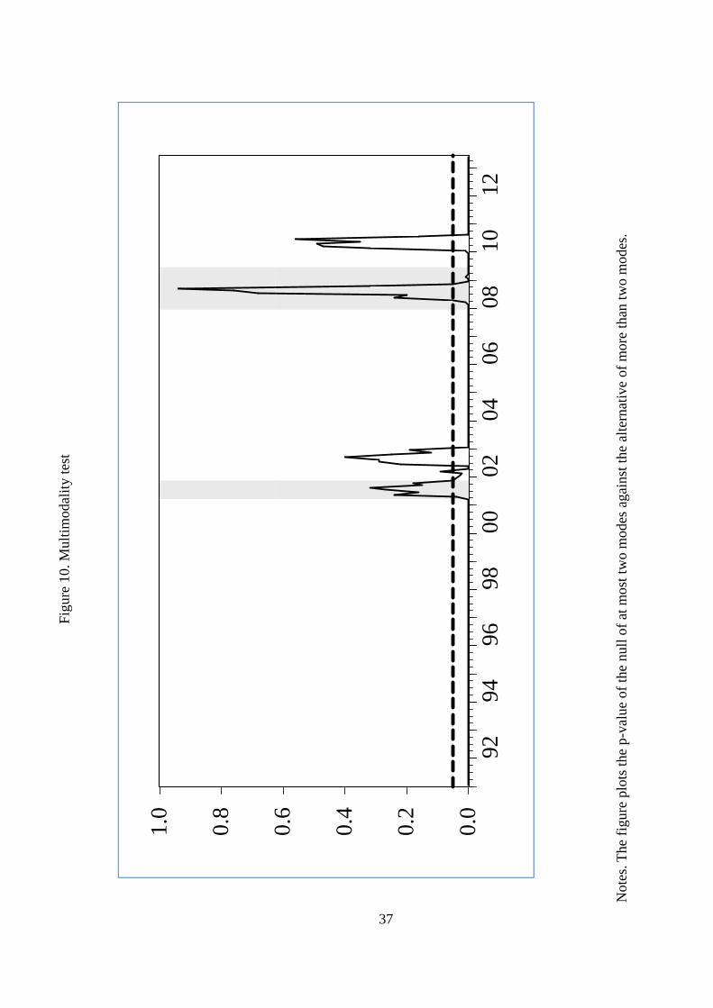
Fig

ure

10. M

ulti

mod

alit

y te

st

1.0

06

0.8

0.4

0.6

0.2

37

0.0

9294

9698

0002

0406

0810

12

Not

es.T

hefi

gure

plot

sth

ep-

valu

eof

the

null

ofat

mos

ttw

om

odes

agai

nstt

heal

tern

ativ

eof

mor

eth

antw

om

odes

.

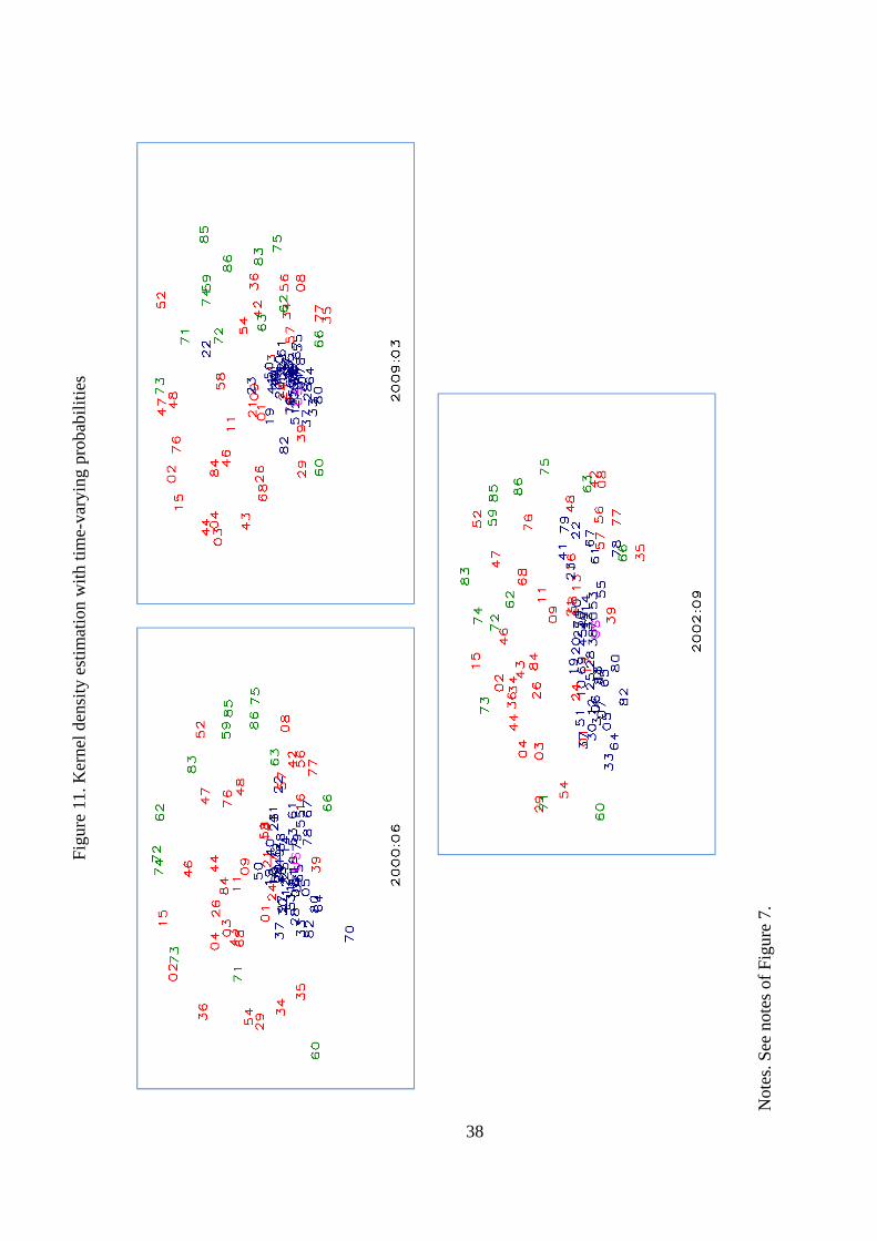
Fig

ure

11. K

erne

l den

sity

est

imat

ion

wit

h ti

me-

vary

ing

prob

abil

itie

s

38

Not

es.S

eeno

tes

ofF

igur

e7.

The propagation of industrial business cyclesThe propagation of industrial business cycles Maximo...

Documents

Transcript of The propagation of industrial business cyclesThe propagation of industrial business cycles Maximo...