Treball Final de Grau - Universitat de Barcelona

Tutor/s

Dra. Elisabet Fuguet Jordà Departament d’Enginyeria Química i

Química Analítica (Secció Química Analítica)

Dra. Clara Ràfols Llach Departament d’Enginyeria Química i

Química Analítica (Secció Química Analítica)

Treball Final de Grau

Optimization of dissolution rate measurements of poor-soluble drugs.

Optimització de les mesures de velocitat de dissolució de fàrmacs amb baixa solubilitat.

Cristina Garcia Marmol June 2019

Aquesta obra esta subjecta a la llicència de: Reconeixement–NoComercial-SenseObraDerivada

http://creativecommons.org/licenses/by-nc-nd/3.0/es/

Agrair a tot el grup de recerca PhysChem pel bon ambient de treball al laboratori, en especial

a la Dra. Elisabet Fuguet Jordà i la Dra. Clara Ràfols Llach per l’ajuda, consells i coneixements

que m’han aportat en tot moment al llarg d’aquests mesos.

A la meva família per recolzar-me en tot moment.

REPORT

Optimization of dissolution rate measurements of poor-soluble drugs. 1

CONTENTS

1. SUMMARY 3

2. RESUM 5

3. INTRODUCTION 7

3.1. Pharmacokinetics 7

3.1.1. Solubility 8

3.1.1.1. pH-Solubility profile 8

3.1.2. Intrinsic dissolution rate 9

3.1.2.1. Methods of IDR measurement 10

3.1.2.2. Miniaturized dissolution methods 11

4. OBJECTIVES 13

5. EXPERIMENTAL SECTION 13

5.1. Reagents and materials 13

5.1.1. GI dissolution method reagents 13

5.1.2. HPLC reagents 13

5.1.3. Studied drugs 14

5.2. Instrumentation 14

5.2.1. GI dissolution method 14

5.2.2. Liquid Chromatography measurements 14

5.3. Procedures 14

5.3.1. Molar extinction coefficients (MEC) and pKas determination 14

5.3.2. Tablet production 15

5.3.3. Dissolution rate measurements 16

5.3.4. Quantification by liquid chromatography 16

5.3.4.1. Extractions 16

5.3.4.2. HPLC 17

2 Garcia Marmol, Cristina

6. TRAZODONE HYDROCHLORIDE 18

6.1. Working conditions optimization 18

6.1.1. Determination of the molar extinction coefficient of trazodone hydrochloride 18

6.1.2. pH 19

6.1.3. Drug weight 20

6.2. Dissolution rate measurements 21

6.2.1. Dissolution rate determined spectrophotometrically without extractions 21

6.2.2. Dissolution rate determined spectrophotometrically with extractions 22

6.2.3. Dissolution rate profiles obtained by off-line quantification 24

7. WARFARIN 27

7.1. Working conditions optimization 27

7.1.1. Determination of the molar extinction coefficient of warfarin 27

7.1.2. pH and drug weight 28

7.1.3. Measurement time 28

7.2. Dissolution rate measurements 29

7.2.1. Dissolution rate determined spectrophotometrically without extractions 30

7.2.2. Dissolution rate determined spectrophotometrically with extractions 31

7.2.3. Dissolution rate profiles obtained by off-line quantification 33

10. CONCLUSIONS 37

11. REFERENCES AND NOTES 39

12. ACRONYMS 41

APPENDICES 43

Appendix 1: Chromatograms 45

Appendix 2: Calibration curves 46


1. SUMMARY

One of the most important parameters to be determined during the drug development process

is the dissolution rate. The in vitro study of this property is essential to evaluate the bioavailability

of drugs in the drug discovery process.

Traditional methods for dissolution rate determination require high amounts of the active

pharmaceutical ingredient. However, it is a problem when drug characterization is carried out in

the early stages of the process, when only little amounts of drug are available. For these reasons,

miniaturized methods, which use low drug amounts, were developed. The gastrointestinal

dissolution method is an example of miniaturized method, and it is used in the present work. The

fact of extracting part of solution at several times, for off-line quantification is not a problem in

traditional methods, because it does not affect the dissolution rate profile curve, as the extracted

volume is not significant compared to the total one. However, that might not be the case in

miniaturized methods, where smaller dissolution volumes are used.

In order to compare the effect of extracting part of solution to quantify off-line the concentration

of drug on the profile curve, dissolution rate measurements have been carried out for 120 minutes

at constant pH for two different drugs: trazodone and warfarin. First, dissolution profiles have been

determined in situ, with spectrophotometric detection. Next, experiments have been repeated

performing several extractions and quantifying off-line by HPLC.

Results show that dissolution profiles are comparable, although the solubility of the

compounds can be a limiting factor.

Determined profiles are similar in the case of trazodone. However, warfarin, with a lower

solubility than trazodone, needs support from a cosolvent to reach equivalent concentrations in

the HPLC profile.

Keywords: Dissolution rate, drug, solubility, active pharmaceutical ingredient, gastrointestinal

dissolution method, trazodone, warfarin, HPLC


2. RESUM

La velocitat de dissolució és un dels paràmetres més importants a determinar durant el procés

de desenvolupament dels fàrmacs. L’estudi in vitro d’aquesta propietat és essencial per avaluar

la biodisponibilitat dels fàrmacs en el seu procés de descobriment.

Per determinar la velocitat de dissolució, els mètodes tradicionals, requereixen quantitats de

principi actiu elevades. No obstant això, suposa un problema quan es fa la caracterització de

fàrmacs en les primeres etapes del procés, quan només hi ha petites quantitats de fàrmacs

disponibles. Per aquests motius, es van desenvolupar mètodes miniaturitzats, els quals utilitzen

quantitats baixes de compost. El gastrointestinal dissolution method és un exemple de mètode

miniaturitzat i ha estat l’utilitzat en aquest treball. El fet d’extreure part de la solució en diverses

ocasions, per a la quantificació off-line no afecta el perfil de la corba, per tant, no suposa un

problema en els mètodes tradicionals, ja que el volum extret no és significatiu en comparació

amb el total. Tanmateix, podria no donar-se el cas en els mètodes miniaturitzats, on s'utilitzen

volums de dissolució més reduïts.

Per comparar com afecta el perfil de la corba, el fet d’extreure part de la solució per quantificar

la concentració de fàrmac off-line, s’han dut a terme mesures de velocitat de dissolució durant

120 minuts a pH constant per a dos fàrmacs diferents: la trazodona i la warfarina. Primer, els

perfils de dissolució s’han determinat in situ, amb detecció espectrofotomètrica. A continuació,

s'han repetit els experiments realitzant diverses extraccions i quantificant-les off-line per HPLC.

Els resultats obtinguts mostren que els perfils de dissolució són comparables, tot i que la

solubilitat dels compostos pot ser un factor limitant.

Els perfils determinats són similars en cas de trazodona. No obstant això, la warfarina, que

té una solubilitat més baixa que la trazodona, necessita el suport d'un cosolvent per arribar a

concentracions equivalents en el perfil de HPLC.

Paraules clau: Velocitat de dissolució, fàrmac, solubilitat, principi actiu, gastrointestinal

dissolution method, trazodona, warfarina, HPLC


3. INTRODUCTION

Many drugs are synthesized by the pharmaceutical industry. The physicochemical

characterization in the early stages of the drug development is a very important step in the drug

discovery process because all those drugs that do not have adequate parameters will not be

further developed. This previous stage allows to save time and money.1 Solubility is one of the

most important parameters because the drug has to be soluble in an aqueous medium2 or has to

be prepared in an appropriate formulation to overcome the limitations of solubility1 to be absorbed.

The other parameter that is very important for the drug development process is the dissolution

rate. This parameter is used to evaluate the stability of drugs and provides information about when

the drug starts working inside the organism.3

However, while solubility is a static concept, which refers to a state of thermodynamic

equilibrium, the dissolution rate responds to a kinetic concept of the process: amount or

concentration of solute that dissolves per unit of time.4 To understand the importance of both

parameters it is necessary to relate them to the pharmacokinetic concept.

3.1. PHARMACOKINETICS

Pharmacokinetics is a pharmacology branch dedicated to the study of how a drug affects an

organism and determines the fate of substances administered to a living organism.5 The

pharmacokinetic process usually explains the ADME properties of a drug which are Absorption,

Distribution, Metabolism, and Excretion. ADME studies provide an estimation of human

pharmacokinetic and metabolic profiles6.

The absorption stage consists of the transfer of a drug from a place of administration to the

blood. The Biopharmaceutics Classification System (BCS) was created based on the

acknowledgement of the importance of solubility and permeability on the fraction absorbed of a

drug.7 It has a regulatory purpose whose underlying idea is that in vitro measurement of solubility,

dissolution, and permeability of drugs in an aqueous medium can predict their in vivo intestinal

absorption.8

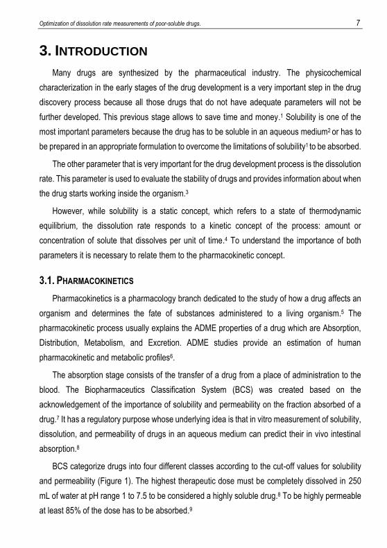
BCS categorize drugs into four different classes according to the cut-off values for solubility

and permeability (Figure 1). The highest therapeutic dose must be completely dissolved in 250

mL of water at pH range 1 to 7.5 to be considered a highly soluble drug.8 To be highly permeable

at least 85% of the dose has to be absorbed.9


Figure 1. Representation of the Biopharmaceutics Classification System.

3.1.1. Solubility

Solubility is the maximum amount of a compound that can be dissolved in a specified volume

of a solvent at a given condition of temperature and pH. It plays a key role in oral absorption

because all drugs should possess an adequate solubility in the gastrointestinal fluids in order to

be able to be absorbed correctly.10

The solubility of a drug depends on many factors and some of them are the hydrophobicity of

the drug molecule and the melting point because it indicates different interactions with the

solvent.11The higher the interaction drug-drug the lower the solubility and dissolution rate of the

compound. However, the pH of the medium is a very important parameter because it affects

ionizable drugs charge state.11

3.1.1.1. pH-Solubility profile

Changes in pH affect the extent of ionization for an ionizable molecule and the relative

proportion of the ionized and unionized drug in solution. Ionizable drugs demonstrate pH

dependence via the Henderson-Hasselbalch solubility profile.11

The profile changes depending on the acid-base character of the compound. However, in

both cases, the lowest solubility is shown when the drug is fully unionized and it is called intrinsic

solubility (S0).11


A B

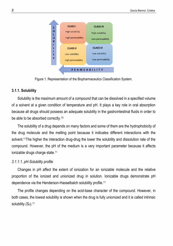
Figure 2. pH solubility profile for a (A) weak base and (B) weak acid.

In Figure 2 the dependence that exists between the solubility and pH can be observed. The

solubility of a weak base (Figure 2A) gets higher when pH decreases. The lowest solubility

appears when the drug is unionized, and the pH is higher than its pKa. Instead, it is observed that

solubility of a weak acid (Figure 2B) gets higher when the pH increases, and the lowest solubility

appears when pH is lower than its pKa. 12

There is a steep increase in the solubility of the molecule as it reaches its pKa and keeps

rising until it reaches pHmax which is the point where the ionizing portion of the curve reaches the

maximum solubility point. This is called a salt plateau. It is the region where the salt form (ionized

molecule associated with a counterion) is in equilibrium with its solid state.11

The counterion effect is significant to determine the solubility constant (Kps). The counterion

associated in the salt form has an opposite charge and it is attracted by columbic interactions.

The interaction strength determines the delimiting solubility.11

3.1.2. Intrinsic Dissolution Rate

The intrinsic dissolution rate is defined as the rate of dissolution of an API under the constant

condition of surface area, pH, temperature and ionic strength.13 The determination of this

parameter helps us understand the solution behaviour of drugs under biophysiological conditions.

The dissolution rate can be expressed by the Noyes-Whitney equation, which fits a first order

exponential Equation 1. From this expression the dissolution rate and an extrapolated solubility

value can be obtained.14


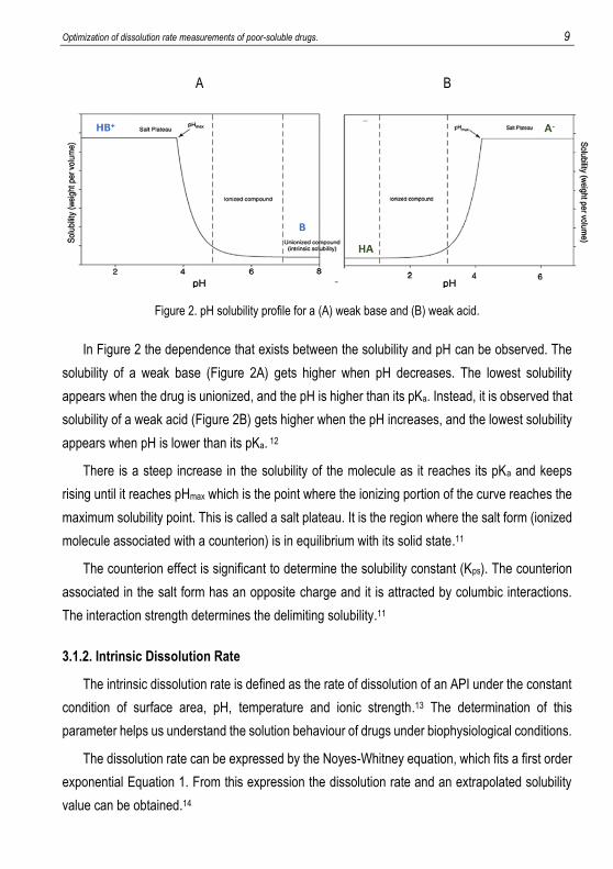
[𝑋]𝑡 = 𝑆 (1 − 𝑒−𝐾𝑑(𝑡−𝑡0)) (1)

[X]t is the weight of the drug in solution in the experiment time (min); S (g) is the extrapolated

solubility of the drug; Kd is the rate constant for dissolution (min-1), and t0 (min) is the measurement

start time.14

Through a refinement process based on the least square adjustment the S, Kd and t0 values

are obtained. The dissolution rate is given by the product Kd . S (g.min-1).14 However, the intrinsic

dissolution rate (IDR) is the product of normalizing the dissolution rate by surface area.

3.1.2.1. Methods of IDR measurement

To evaluate the bioavailability of Active Pharmaceutical Ingredients (APIs) it is important to

carry out dissolution rate tests. Three different methods exist to perform the dissolution rate (DR)

measurements, mainly differentiated by the way the drug is added to the dissolution vial. DR is

typically measured using a rotating or static disc of compacted powder (disc method) where the

drug powder is compacted on a disc which has a defined surface area. In addition, disc method

is usually used for drugs with an apparent solubility Sapp> 1mg/mL.9 Other not so common

methods are the coarse powder, where the solid compound is added directly to the vial, and the

suspensions method, where a controlled particle size of powder drug is dispersed. In contrast to

disc method, coarse powder and suspensions method are more commonly used for drugs with a

lower apparent solubility (Sapp<100 µg/ mL) 9 because the surface area which is in contact with

the dissolution medium is higher and it speeds up the dissolution of the drug. However, apparent

solubility is not considered a limiting parameter to decide which method has to be used.

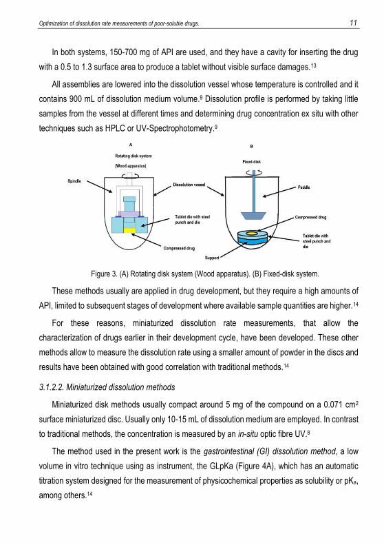
Pharmacopoeias list two types of traditional apparatus to determine the dissolution rate; A

rotating disc system which uses United States Pharmacopeia (USP) Wood Apparatus (Wood

method) (Figure 3A), where drug dissolution is carried out by a rotating force system on spindle

which is fitted to the tablet die (Figure 3A). API is compressed in a steel punch and die (Figure

3A), and the obtained tablet must be smooth and free of visible defects with a 0.5 cm2 to 1.3 cm2

of surface area.8 The compound disc is then fitted to a rotational assembly in a dissolution bath

as shown in the Figure 3A.13The other traditional apparatus is the fixed-disc system (Figure 3B)

where as Wood method, the compacted drug is inside a pellet and die assembly (Figure 3B),

however, in this system, the assembly is fixed, and the dissolution is achieved by moving the

volume of dissolution medium with a paddle apparatus over the disc (Figure 3B).13


In both systems, 150-700 mg of API are used, and they have a cavity for inserting the drug

with a 0.5 to 1.3 surface area to produce a tablet without visible surface damages.13

All assemblies are lowered into the dissolution vessel whose temperature is controlled and it

contains 900 mL of dissolution medium volume.9 Dissolution profile is performed by taking little

samples from the vessel at different times and determining drug concentration ex situ with other

techniques such as HPLC or UV-Spectrophotometry.9

Figure 3. (A) Rotating disk system (Wood apparatus). (B) Fixed-disk system.

These methods usually are applied in drug development, but they require a high amounts of

API, limited to subsequent stages of development where available sample quantities are higher.14

For these reasons, miniaturized dissolution rate measurements, that allow the

characterization of drugs earlier in their development cycle, have been developed. These other

methods allow to measure the dissolution rate using a smaller amount of powder in the discs and

results have been obtained with good correlation with traditional methods.14

3.1.2.2. Miniaturized dissolution methods

Miniaturized disk methods usually compact around 5 mg of the compound on a 0.071 cm2

surface miniaturized disc. Usually only 10-15 mL of dissolution medium are employed. In contrast

to traditional methods, the concentration is measured by an in-situ optic fibre UV.8

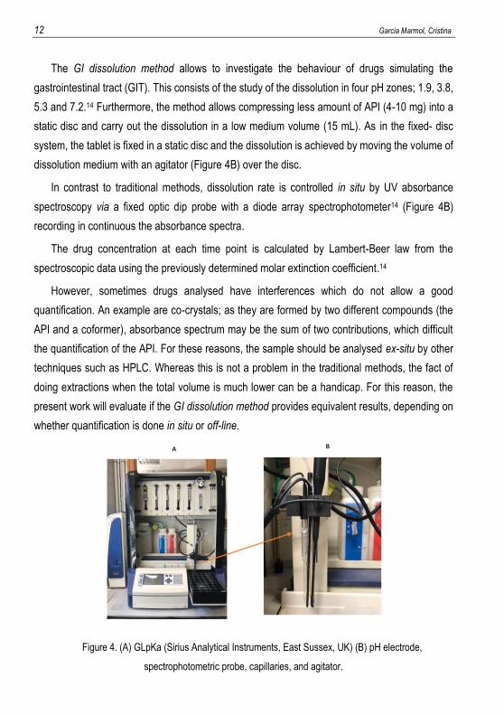
The method used in the present work is the gastrointestinal (GI) dissolution method, a low

volume in vitro technique using as instrument, the GLpKa (Figure 4A), which has an automatic

titration system designed for the measurement of physicochemical properties as solubility or pKa,

among others.14


The GI dissolution method allows to investigate the behaviour of drugs simulating the

gastrointestinal tract (GIT). This consists of the study of the dissolution in four pH zones; 1.9, 3.8,

5.3 and 7.2.14 Furthermore, the method allows compressing less amount of API (4-10 mg) into a

static disc and carry out the dissolution in a low medium volume (15 mL). As in the fixed- disc

system, the tablet is fixed in a static disc and the dissolution is achieved by moving the volume of

dissolution medium with an agitator (Figure 4B) over the disc.

In contrast to traditional methods, dissolution rate is controlled in situ by UV absorbance

spectroscopy via a fixed optic dip probe with a diode array spectrophotometer14 (Figure 4B)

recording in continuous the absorbance spectra.

The drug concentration at each time point is calculated by Lambert-Beer law from the

spectroscopic data using the previously determined molar extinction coefficient.14

However, sometimes drugs analysed have interferences which do not allow a good

quantification. An example are co-crystals; as they are formed by two different compounds (the

API and a coformer), absorbance spectrum may be the sum of two contributions, which difficult

the quantification of the API. For these reasons, the sample should be analysed ex-situ by other

techniques such as HPLC. Whereas this is not a problem in the traditional methods, the fact of

doing extractions when the total volume is much lower can be a handicap. For this reason, the

present work will evaluate if the GI dissolution method provides equivalent results, depending on

whether quantification is done in situ or off-line.

Figure 4. (A) GLpKa (Sirius Analytical Instruments, East Sussex, UK) (B) pH electrode,

spectrophotometric probe, capillaries, and agitator.


4. OBJECTIVES

Traditional methods for measuring dissolution rate of drugs use high sample amounts and

volumes, for this reason the fact of extracting part of the solution to determine the concentration

of drug does not affect the curve of the dissolution rate. In contrast, in the GI dissolution method

the volumes are very small, and extracting a quantity of solution may affect more in the obtained

dissolution rate.

The objective is to study how doing extractions in a low volume dissolution apparatus affects

the dissolution rate and check if there is any difference between the dissolution rate curve

analysed by the GI dissolution method or by HPLC.

Also, another objective is to determine to which extent drug solubility limits the quantification

off-line by HPLC.

5. EXPERIMENTAL SECTION

5.1. REAGENTS AND MATERIALS

5.1.1. GI dissolution method reagents

In the preparation of the pH 1.6 buffer for the GI dissolution method the following chemicals

were used: sodium acetate anhydrous (99,6%) from J.T. Backer (Deventer, Holland)), potassium

dihydrogen phosphate (>99,5%) and 0.5 M hydrochloric acid solution from Merck (Darmstadt,

Germany). pH was measured with pH meter Crison GLP22 (Italy). Water was purified by a Mili-Q

plus system from Millipore (Bedford, MA, USA) with a resistivity of 18.2 MΩ . cm.

In the GI dissolution method, the following chemicals were used: 0.15 M potassium chloride

(99.5%) (ISA water), DMSO (99,8%) and Titrisol® solutions of 0.5 M potassium hydroxide and

0.5 M hydrochloric acid all from Merck.

5.1.2. HPLC reagents

The methanol (HPLC grade) used for the HPLC mobile phase was from Thermo Fisher

Scientific U.K.


In the preparation of the buffers for the HPLC mobile phase, the following chemicals were

used: formic acid (98%), sodium hydroxide (>99%) both from Merck, formic acid (85%) from Carlo

Erba and acetic acid (99-100%) from J.T. Backer.

5.1.1. Studied drugs

The drugs used were trazodone hydrochloride (>99%) and warfarin (>98%) both from Sigma

Aldrich, Germany.

5.2. INSTRUMENTATION

5.2.1. GI dissolution method

The apparatus used to measure the molar extinction coefficients, pKas and the dissolution

rate was GLpKa (Sirius Analytical Instruments, East Sussex, UK) equipped with a fibre optic dip

probe with a diode array spectrometer D-PAS (Dip Probe Absorption Spectroscopy). The

apparatus was controlled from a computer running the RefinementPro2 software and the data

refinement was completed with Sirius T3 Refine.

All measurements were performed at room temperature in 0.15 M KCl solution (ISA Water)

using standardized 0.5 M KOH and 0.5 M HCl solutions. The measured pH range was from 1.8

to 12.2.

5.2.2. Liquid Chromatography measurements

A Schimadzu liquid chromatograph equipped with two Shimadzy LC-10AD VP pumps and a

Shimadzu SPD-10AV VP UV-VIS detector was used for the quantification of samples.

The apparatus was controlled from a computer running the LC solutions software from

Shimadzu.

5.3. PROCEDURES

5.3.1. Molar extinction coefficients (MEC) and pKas determination

The molar extinction coefficients for neutral and ionized form of drugs and pKas were

determined by UV- metric titration using the instrument GLpKa (Figure 4) in aqueous medium.


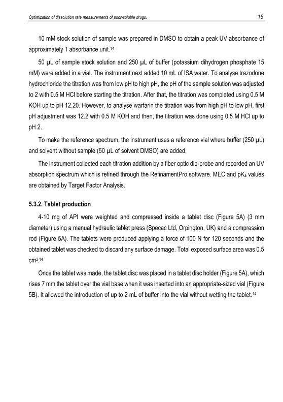
10 mM stock solution of sample was prepared in DMSO to obtain a peak UV absorbance of

approximately 1 absorbance unit.14

50 µL of sample stock solution and 250 µL of buffer (potassium dihydrogen phosphate 15

mM) were added in a vial. The instrument next added 10 mL of ISA water. To analyse trazodone

hydrochloride the titration was from low pH to high pH, the pH of the sample solution was adjusted

to 2 with 0.5 M HCl before starting the titration. After that, the titration was completed using 0.5 M

KOH up to pH 12.20. However, to analyse warfarin the titration was from high pH to low pH, first

pH adjustment was 12.2 with 0.5 M KOH and then, the titration was done using 0.5 M HCl up to

pH 2.

To make the reference spectrum, the instrument uses a reference vial where buffer (250 µL)

and solvent without sample (50 µL of solvent DMSO) are added.

The instrument collected each titration addition by a fiber optic dip-probe and recorded an UV

absorption spectrum which is refined through the RefinamentPro software. MEC and pKa values

are obtained by Target Factor Analysis.

5.3.2. Tablet production

4-10 mg of API were weighted and compressed inside a tablet disc (Figure 5A) (3 mm

diameter) using a manual hydraulic tablet press (Specac Ltd, Orpington, UK) and a compression

rod (Figure 5A). The tablets were produced applying a force of 100 N for 120 seconds and the

obtained tablet was checked to discard any surface damage. Total exposed surface area was 0.5

cm2.14

Once the tablet was made, the tablet disc was placed in a tablet disc holder (Figure 5A), which

rises 7 mm the tablet over the vial base when it was inserted into an appropriate-sized vial (Figure

5B). It allowed the introduction of up to 2 mL of buffer into the vial without wetting the tablet.14


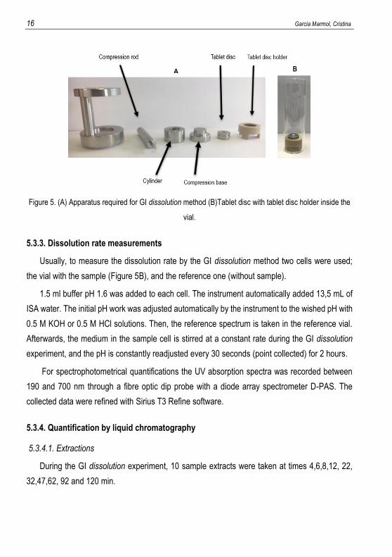
Figure 5. (A) Apparatus required for GI dissolution method (B)Tablet disc with tablet disc holder inside the

vial.

5.3.3. Dissolution rate measurements

Usually, to measure the dissolution rate by the GI dissolution method two cells were used;

the vial with the sample (Figure 5B), and the reference one (without sample).

1.5 ml buffer pH 1.6 was added to each cell. The instrument automatically added 13,5 mL of

ISA water. The initial pH work was adjusted automatically by the instrument to the wished pH with

0.5 M KOH or 0.5 M HCl solutions. Then, the reference spectrum is taken in the reference vial.

Afterwards, the medium in the sample cell is stirred at a constant rate during the GI dissolution

experiment, and the pH is constantly readjusted every 30 seconds (point collected) for 2 hours.

For spectrophotometrical quantifications the UV absorption spectra was recorded between

190 and 700 nm through a fibre optic dip probe with a diode array spectrometer D-PAS. The

collected data were refined with Sirius T3 Refine software.

5.3.4. Quantification by liquid chromatography

5.3.4.1. Extractions

During the GI dissolution experiment, 10 sample extracts were taken at times 4,6,8,12, 22,

32,47,62, 92 and 120 min.


A sample of 50 µL was extracted, initially in very small intervals of time to study in detail the

evolution of the dissolution rate. However, when the dissolution experiment evolved, the time

intervals were larger because there were fewer changes in solution concentration.

In case that drug solubility was extremely low, the samples extracts were dissolved in 50 µL

of methanol to keep all the drug in solution and avoid precipitation.

5.3.4.2. HPLC

First, the calibration curves for each drug were carried out. The solvent used to prepare the

standard solutions was the same as the mobile phase used in the chromatographic conditions.

The study of all the drugs was carried out in isocratic conditions using Symmetry® C8

4.6x50mm, 5µm column without precolumn and at the maximum absorption wavelength in order

to obtain the maximum signal. Two examples of chromatograms are shown in Appendix 1 and

two examples of calibration curves are shown in Appendix 2.

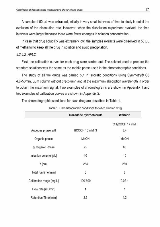
The chromatographic conditions for each drug are described in Table 1.

Table 1. Chromatographic conditions for each studied drug.

Trazodone hydrochloride Warfarin

Aqueous phase; pH HCOOH 10 mM; 3

CH3COOH 17 mM;

3.4

Organic phase MeOH MeOH

% Organic Phase 25 60

Injection volume [L] 10 10

λ [nm] 254 280

Total run time [min] 5 6

Calibration range [mg/L] 100-600 0.02-1

Flow rate [mL/min] 1 1

Retention Time [min] 2.3 4.2


6. TRAZODONE HYDROCHLORIDE

Trazodone is an antidepressant derivative of triazolopyridine which works as an inhibitor of

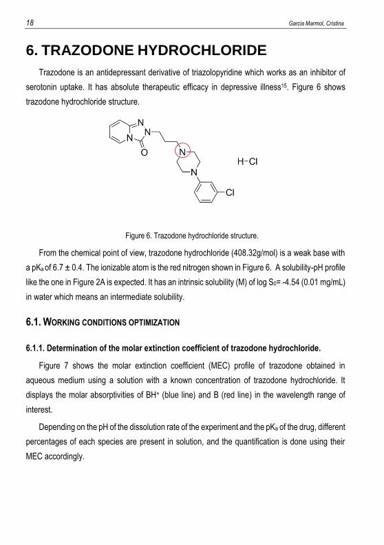
serotonin uptake. It has absolute therapeutic efficacy in depressive illness15. Figure 6 shows

trazodone hydrochloride structure.

Figure 6. Trazodone hydrochloride structure.

From the chemical point of view, trazodone hydrochloride (408.32g/mol) is a weak base with

a pKa of 6.7 ± 0.4. The ionizable atom is the red nitrogen shown in Figure 6. A solubility-pH profile

like the one in Figure 2A is expected. It has an intrinsic solubility (M) of log S0= -4.54 (0.01 mg/mL)

in water which means an intermediate solubility.

6.1. WORKING CONDITIONS OPTIMIZATION

6.1.1. Determination of the molar extinction coefficient of trazodone hydrochloride.

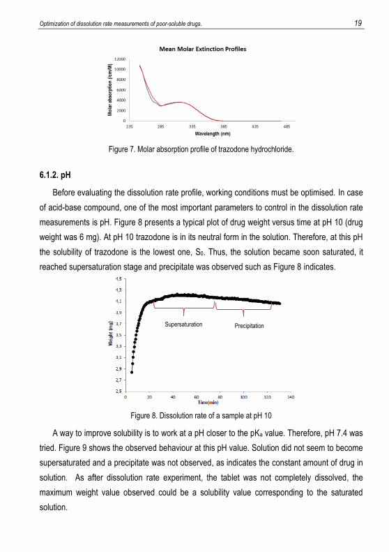
Figure 7 shows the molar extinction coefficient (MEC) profile of trazodone obtained in

aqueous medium using a solution with a known concentration of trazodone hydrochloride. It

displays the molar absorptivities of BH+ (blue line) and B (red line) in the wavelength range of

interest.

Depending on the pH of the dissolution rate of the experiment and the pKa of the drug, different

percentages of each species are present in solution, and the quantification is done using their

MEC accordingly.


Figure 7. Molar absorption profile of trazodone hydrochloride.

6.1.2. pH

Before evaluating the dissolution rate profile, working conditions must be optimised. In case

of acid-base compound, one of the most important parameters to control in the dissolution rate

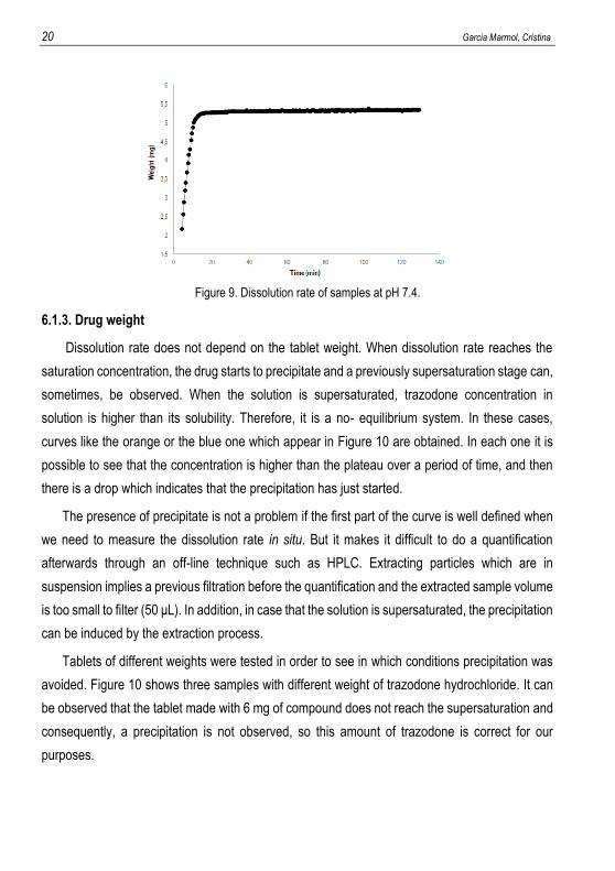
measurements is pH. Figure 8 presents a typical plot of drug weight versus time at pH 10 (drug

weight was 6 mg). At pH 10 trazodone is in its neutral form in the solution. Therefore, at this pH

the solubility of trazodone is the lowest one, S0. Thus, the solution became soon saturated, it

reached supersaturation stage and precipitate was observed such as Figure 8 indicates.

Figure 8. Dissolution rate of a sample at pH 10

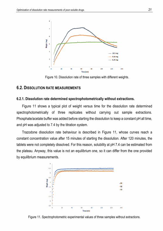
A way to improve solubility is to work at a pH closer to the pKa value. Therefore, pH 7.4 was

tried. Figure 9 shows the observed behaviour at this pH value. Solution did not seem to become

supersaturated and a precipitate was not observed, as indicates the constant amount of drug in

solution. As after dissolution rate experiment, the tablet was not completely dissolved, the

maximum weight value observed could be a solubility value corresponding to the saturated

solution.

Supersaturation Precipitation


Figure 9. Dissolution rate of samples at pH 7.4.

6.1.3. Drug weight

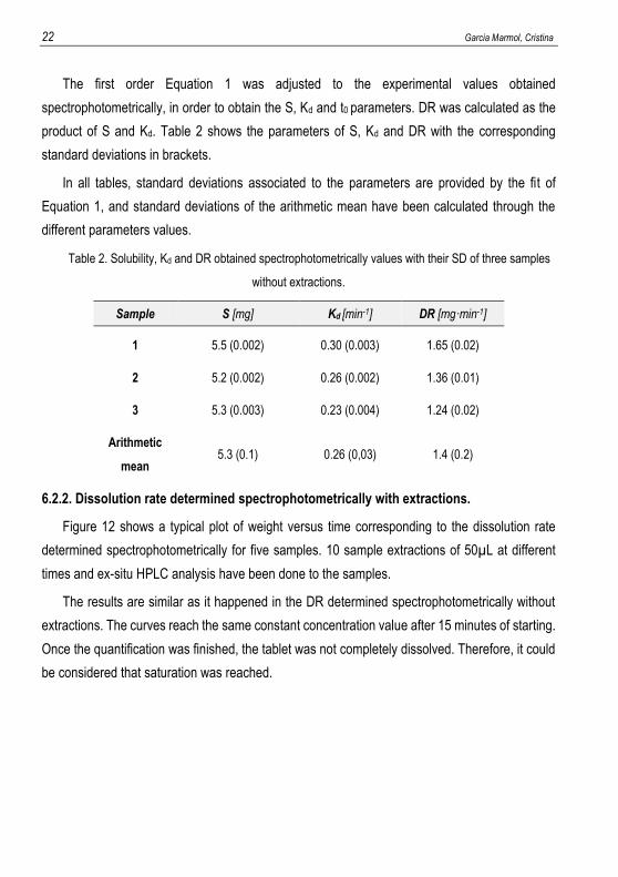
Dissolution rate does not depend on the tablet weight. When dissolution rate reaches the

saturation concentration, the drug starts to precipitate and a previously supersaturation stage can,

sometimes, be observed. When the solution is supersaturated, trazodone concentration in

solution is higher than its solubility. Therefore, it is a no- equilibrium system. In these cases,

curves like the orange or the blue one which appear in Figure 10 are obtained. In each one it is

possible to see that the concentration is higher than the plateau over a period of time, and then

there is a drop which indicates that the precipitation has just started.

The presence of precipitate is not a problem if the first part of the curve is well defined when

we need to measure the dissolution rate in situ. But it makes it difficult to do a quantification

afterwards through an off-line technique such as HPLC. Extracting particles which are in

suspension implies a previous filtration before the quantification and the extracted sample volume

is too small to filter (50 μL). In addition, in case that the solution is supersaturated, the precipitation

can be induced by the extraction process.

Tablets of different weights were tested in order to see in which conditions precipitation was

avoided. Figure 10 shows three samples with different weight of trazodone hydrochloride. It can

be observed that the tablet made with 6 mg of compound does not reach the supersaturation and

consequently, a precipitation is not observed, so this amount of trazodone is correct for our

purposes.


Figure 10. Dissolution rate of three samples with different weights.

6.2. DISSOLUTION RATE MEASUREMENTS

6.2.1. Dissolution rate determined spectrophotometrically without extractions.

Figure 11 shows a typical plot of weight versus time for the dissolution rate determined

spectrophotometrically of three replicates without carrying out sample extractions.

Phosphate/acetate buffer was added before starting the dissolution to keep a constant pH all time,

and pH was adjusted to 7.4 by the titration system.

Trazodone dissolution rate behaviour is described in Figure 11, whose curves reach a

constant concentration value after 15 minutes of starting the dissolution. After 120 minutes, the

tablets were not completely dissolved. For this reason, solubility at pH 7.4 can be estimated from

the plateau. Anyway, this value is not an equilibrium one, so it can differ from the one provided

by equilibrium measurements.

Figure 11. Spectrophotometric experimental values of three samples without extractions.


The first order Equation 1 was adjusted to the experimental values obtained

spectrophotometrically, in order to obtain the S, Kd and t0 parameters. DR was calculated as the

product of S and Kd. Table 2 shows the parameters of S, Kd and DR with the corresponding

standard deviations in brackets.

In all tables, standard deviations associated to the parameters are provided by the fit of

Equation 1, and standard deviations of the arithmetic mean have been calculated through the

different parameters values.

Table 2. Solubility, Kd and DR obtained spectrophotometrically values with their SD of three samples

without extractions.

6.2.2. Dissolution rate determined spectrophotometrically with extractions.

Figure 12 shows a typical plot of weight versus time corresponding to the dissolution rate

determined spectrophotometrically for five samples. 10 sample extractions of 50µL at different

times and ex-situ HPLC analysis have been done to the samples.

The results are similar as it happened in the DR determined spectrophotometrically without

extractions. The curves reach the same constant concentration value after 15 minutes of starting.

Once the quantification was finished, the tablet was not completely dissolved. Therefore, it could

be considered that saturation was reached.

Sample S [mg] Kd [min-1] DR [mg·min-1]

1 5.5 (0.002) 0.30 (0.003) 1.65 (0.02)

2 5.2 (0.002) 0.26 (0.002) 1.36 (0.01)

3 5.3 (0.003) 0.23 (0.004) 1.24 (0.02)

Arithmetic

mean 5.3 (0.1) 0.26 (0,03) 1.4 (0.2)


Figure 12. Spectrophotometrically experimental values of five samples with extractions.

Table 3 shows the obtained parameter of S, Kd and DR with its standard deviations.

Table 3. Solubility, Kd and DR obtained spectrophotometrically values with their SD of five samples

with extractions.

Comparing DR value doing extractions 1.7 (0.4) mg.min-1 (Table 3) and without doing

extractions 1.4 (0.2) mg.min-1 (Table 2), there are no significant differences between them. In

order to compare if both procedures are equivalent to each other, Figure 13 shows the average

curve profile doing and not doing extractions. The orange profile represents the average

experimental points of dissolution rate with the standard deviations as error bars when extractions

are done. The blue one represents the experimental values analysed spectrophotometrically

without carrying out extractions also with the error bars. Figure 13 proves the fact that doing 10

extractions of 50µL does not affect considerably the curve of dissolution rate, as both curves

overlap.


1 5.41 (0.003) 0.40 (0.007) 2.17 (0.04)

2 5.42 (0.003) 0.24 (0.003) 1.28 (0.02)

3 5.33 (0.003) 0.31 (0.004) 1.64 (0.02)

4 5.41 (0.002) 0.39 (0.004) 2.09 (0.02)

5 5.35 (0.004) 0.32 (0.006) 1.72 (0.03)

Arithmetic mean 5.38 (0.04) 0.31 (0.07) 1.7 (0.4)


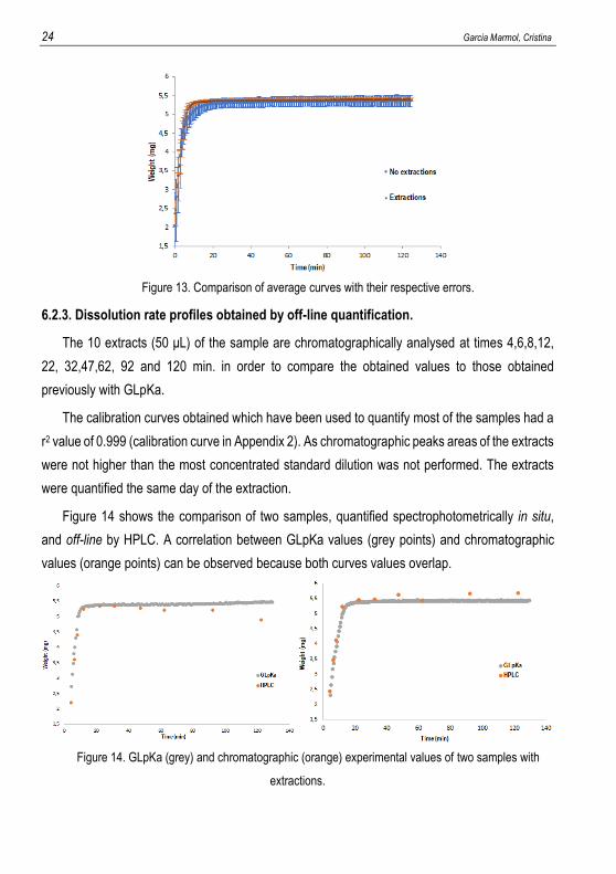
Figure 13. Comparison of average curves with their respective errors.

6.2.3. Dissolution rate profiles obtained by off-line quantification.

The 10 extracts (50 μL) of the sample are chromatographically analysed at times 4,6,8,12,

22, 32,47,62, 92 and 120 min. in order to compare the obtained values to those obtained

previously with GLpKa.

The calibration curves obtained which have been used to quantify most of the samples had a

r2 value of 0.999 (calibration curve in Appendix 2). As chromatographic peaks areas of the extracts

were not higher than the most concentrated standard dilution was not performed. The extracts

were quantified the same day of the extraction.

Figure 14 shows the comparison of two samples, quantified spectrophotometrically in situ,

and off-line by HPLC. A correlation between GLpKa values (grey points) and chromatographic

values (orange points) can be observed because both curves values overlap.

Figure 14. GLpKa (grey) and chromatographic (orange) experimental values of two samples with

extractions.


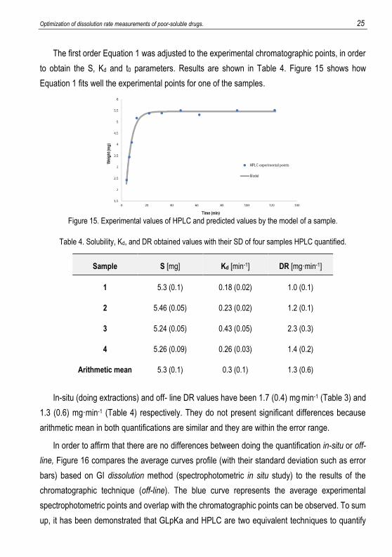
The first order Equation 1 was adjusted to the experimental chromatographic points, in order

to obtain the S, Kd and t0 parameters. Results are shown in Table 4. Figure 15 shows how

Equation 1 fits well the experimental points for one of the samples.

Figure 15. Experimental values of HPLC and predicted values by the model of a sample.

Table 4. Solubility, Kd, and DR obtained values with their SD of four samples HPLC quantified.

In-situ (doing extractions) and off- line DR values have been 1.7 (0.4) mg.min-1 (Table 3) and

1.3 (0.6) mg·min-1 (Table 4) respectively. They do not present significant differences because

arithmetic mean in both quantifications are similar and they are within the error range.

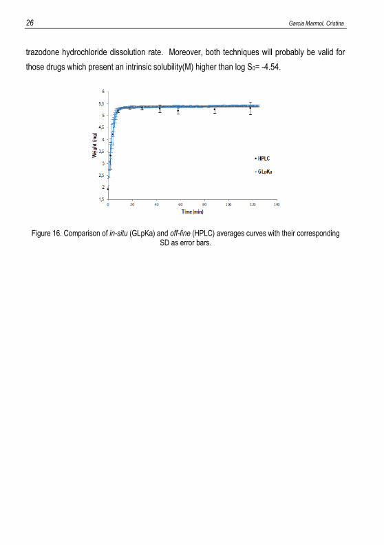
In order to affirm that there are no differences between doing the quantification in-situ or off-

line, Figure 16 compares the average curves profile (with their standard deviation such as error

bars) based on GI dissolution method (spectrophotometric in situ study) to the results of the

chromatographic technique (off-line). The blue curve represents the average experimental

spectrophotometric points and overlap with the chromatographic points can be observed. To sum

up, it has been demonstrated that GLpKa and HPLC are two equivalent techniques to quantify


1 5.3 (0.1) 0.18 (0.02) 1.0 (0.1)

2 5.46 (0.05) 0.23 (0.02) 1.2 (0.1)

3 5.24 (0.05) 0.43 (0.05) 2.3 (0.3)

4 5.26 (0.09) 0.26 (0.03) 1.4 (0.2)

Arithmetic mean 5.3 (0.1) 0.3 (0.1) 1.3 (0.6)


trazodone hydrochloride dissolution rate. Moreover, both techniques will probably be valid for

those drugs which present an intrinsic solubility(M) higher than log S0= -4.54.

Figure 16. Comparison of in-situ (GLpKa) and off-line (HPLC) averages curves with their corresponding SD as error bars.


7. WARFARIN

Warfarin is an anticoagulant which works as an inhibitor of the vitamin K production, reducing

the ability of the blood to clot.16 Figure 17 shows warfarin structure.

Figure 17. Warfarin structure

From the chemical point of view, warfarin (308.34 g/mol) is a weak acid with a pKa of 4.9±0.4.

The ionizable atom is the red oxygen shown in Figure 17. A solubility-pH profile like the one Figure

2B is expected. It has an intrinsic solubility (M) of log S0= -4.33 (6 µg/mL) in water which means

a poor solubility.

7.1. WORKING CONDITIONS OPTIMIZATION

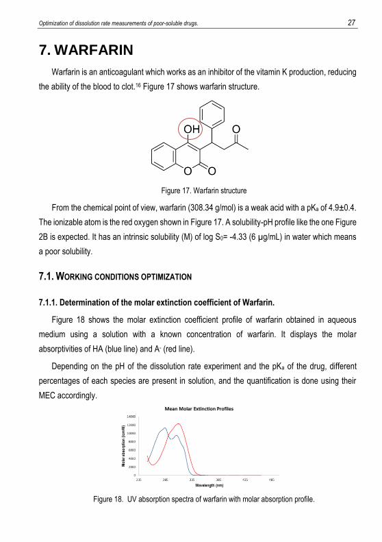
7.1.1. Determination of the molar extinction coefficient of Warfarin.

Figure 18 shows the molar extinction coefficient profile of warfarin obtained in aqueous

medium using a solution with a known concentration of warfarin. It displays the molar

absorptivities of HA (blue line) and A- (red line).

Depending on the pH of the dissolution rate experiment and the pKa of the drug, different

percentages of each species are present in solution, and the quantification is done using their

MEC accordingly.

Figure 18. UV absorption spectra of warfarin with molar absorption profile.


7.1.2. pH and drug weight

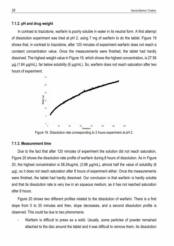
In contrast to trazodone, warfarin is poorly soluble in water in its neutral form. A first attempt

of dissolution experiment was tried at pH 2, using 7 mg of warfarin to do the tablet. Figure 19

shows that, in contrast to trazodone, after 120 minutes of experiment warfarin does not reach a

constant concentration value. Once the measurements were finished, the tablet had hardly

dissolved. The highest weight value in Figure 19, which shows the highest concentration, is 27.56

µg (1.84 µg/mL), far below solubility (6 µg/mL). So, warfarin does not reach saturation after two

hours of experiment.

Figure 19. Dissolution rate corresponding to 2 hours experiment at pH 2.

7.1.3. Measurement time

Due to the fact that after 120 minutes of experiment the solution did not reach saturation,

Figure 20 shows the dissolution rate profile of warfarin during 8 hours of dissolution. As in Figure

20, the highest concentration is 58.24ug/mL (3.88 µg/mL), almost half the value of solubility (6

µg), so it does not reach saturation after 8 hours of experiment either. Once the measurements

were finished, the tablet had hardly dissolved. Our conclusion is that warfarin is hardly soluble

and that its dissolution rate is very low in an aqueous medium, as it has not reached saturation

after 8 hours.

Figure 20 shows two different profiles related to the dissolution of warfarin. There is a first

slope from 0 to 20 minutes and then, slope decreases, and a second dissolution profile is

observed. This could be due to two phenomena:

- Warfarin is difficult to press as a solid. Usually, some particles of powder remained

attached to the disc around the tablet and it was difficult to remove them. Its dissolution


would present a higher DR than the tablet DR, because the superficial area of the

particles is higher, and consequently, so is the dissolution rate (powder coarse method).

- The crystalline structure of the tablet might change during the dissolution process, which

would result in two different DR, the first one would be caused by the initial warfarin’s

solid, and the second one to the change of crystalline structure in the tablet. In order to

prove this, an x-ray analysis of warfarin powder and solid tablet after DR measurement

should be performed.

Figure 20 shows a fit of Equation (1) to the experimental points corresponding to the first 20

minutes of dissolution (green). The obtained dissolution rate is 3.1 (0.2) µg·min-1. The blue curve

belongs to the fit of the second profile, which gives a dissolution rate of 0.302 (0.002) µg·min-1.

Figure 20. Dissolution rate corresponding to 8 hours experiment at pH 2. Orange: Experimental points

Green: fit of the first 20 minutes of dissolution. Blue: fit of the rest of the curve.

After these preliminary experiments, tablets of 6-7 mg were done for the rest of experimental,

and pH 2 was selected as an appropriate pH, as our objective was to work with a compound with

much lower solubility than trazodone.

Dissolution rate experiments were 120 minutes long and in case that two profiles were

observed, the whole curve was fitted to Equation 1.

7.2. DISSOLUTION RATE MEASUREMENTS

Phosphate/acetate buffer was added before starting the dissolution to keep a constant pH all

time, and pH was adjusted to 2 by the titration system. The experiments were carried in two

different ways: DR determined spectrophotometrically (in-situ) without doing exactions and with

doing it. The extracts were analysed off-line by HPLC in order to compare the results.


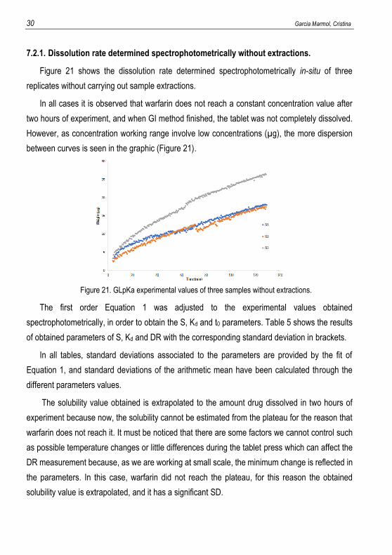
7.2.1. Dissolution rate determined spectrophotometrically without extractions.

Figure 21 shows the dissolution rate determined spectrophotometrically in-situ of three

replicates without carrying out sample extractions.

In all cases it is observed that warfarin does not reach a constant concentration value after

two hours of experiment, and when GI method finished, the tablet was not completely dissolved.

However, as concentration working range involve low concentrations (µg), the more dispersion

between curves is seen in the graphic (Figure 21).

Figure 21. GLpKa experimental values of three samples without extractions.

The first order Equation 1 was adjusted to the experimental values obtained

spectrophotometrically, in order to obtain the S, Kd and t0 parameters. Table 5 shows the results

of obtained parameters of S, Kd and DR with the corresponding standard deviation in brackets.

In all tables, standard deviations associated to the parameters are provided by the fit of

Equation 1, and standard deviations of the arithmetic mean have been calculated through the

different parameters values.

The solubility value obtained is extrapolated to the amount drug dissolved in two hours of

experiment because now, the solubility cannot be estimated from the plateau for the reason that

warfarin does not reach it. It must be noticed that there are some factors we cannot control such

as possible temperature changes or little differences during the tablet press which can affect the

DR measurement because, as we are working at small scale, the minimum change is reflected in

the parameters. In this case, warfarin did not reach the plateau, for this reason the obtained

solubility value is extrapolated, and it has a significant SD.


Table 5. Solubility, Kd and DR values with their SD of three samples without extractions.

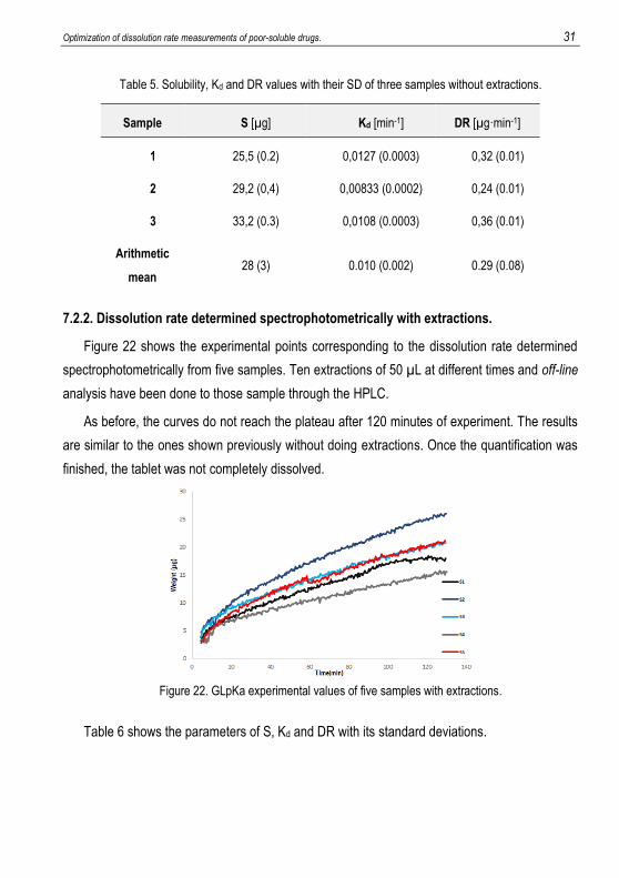
7.2.2. Dissolution rate determined spectrophotometrically with extractions.

Figure 22 shows the experimental points corresponding to the dissolution rate determined

spectrophotometrically from five samples. Ten extractions of 50 µL at different times and off-line

analysis have been done to those sample through the HPLC.

As before, the curves do not reach the plateau after 120 minutes of experiment. The results

are similar to the ones shown previously without doing extractions. Once the quantification was

finished, the tablet was not completely dissolved.

Figure 22. GLpKa experimental values of five samples with extractions.

Table 6 shows the parameters of S, Kd and DR with its standard deviations.

Sample S [µg] Kd [min-1] DR [µg·min-1]

1 25,5 (0.2) 0,0127 (0.0003) 0,32 (0.01)

2 29,2 (0,4) 0,00833 (0.0002) 0,24 (0.01)

3 33,2 (0.3) 0,0108 (0.0003) 0,36 (0.01)

Arithmetic

mean 28 (3) 0.010 (0.002) 0.29 (0.08)


Table 6. Solubility, Kd and DR obtained spectrophotometrically values with their SD of five samples with

extractions.

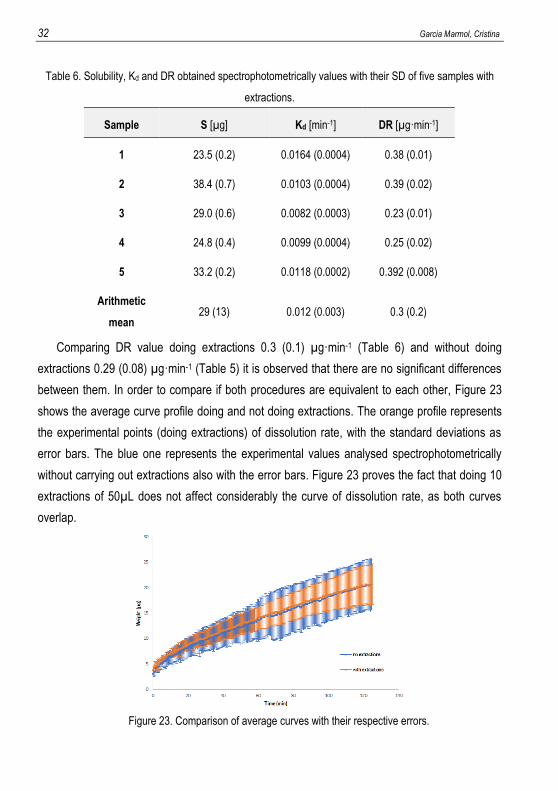
Comparing DR value doing extractions 0.3 (0.1) µg·min-1 (Table 6) and without doing

extractions 0.29 (0.08) µg·min-1 (Table 5) it is observed that there are no significant differences

between them. In order to compare if both procedures are equivalent to each other, Figure 23

shows the average curve profile doing and not doing extractions. The orange profile represents

the experimental points (doing extractions) of dissolution rate, with the standard deviations as

error bars. The blue one represents the experimental values analysed spectrophotometrically

without carrying out extractions also with the error bars. Figure 23 proves the fact that doing 10

extractions of 50µL does not affect considerably the curve of dissolution rate, as both curves

overlap.

Figure 23. Comparison of average curves with their respective errors.


1 23.5 (0.2) 0.0164 (0.0004) 0.38 (0.01)

2 38.4 (0.7) 0.0103 (0.0004) 0.39 (0.02)

3 29.0 (0.6) 0.0082 (0.0003) 0.23 (0.01)

4 24.8 (0.4) 0.0099 (0.0004) 0.25 (0.02)

5 33.2 (0.2) 0.0118 (0.0002) 0.392 (0.008)

Arithmetic

mean 29 (13) 0.012 (0.003) 0.3 (0.2)


7.2.3. Dissolution rate profiles obtained by off-line quantification.

The 10 extracts (50 μL) of the sample are chromatographically analysed in order to compare

the obtained values to those obtained previously with GLpKa.

The calibration curves obtained which have been used to quantify most of the samples had a

r2 value of 0.999 (calibration curve in Appendix 2). As chromatographic peaks areas of the extracts

were not considerably higher than the most concentrated standard, dilution was not performed.

The extracts were quantified the same day of the extraction.

Figure 24A shows the techniques (HPLC and spectroscopic values) comparison for one

sample. Chromatographic values are below those obtained spectrophotometrically. This might be

due to the appearance of a precipitate which could be caused by the manipulation of the solution

during the extraction process. To prove this, the samples, immediately after each extraction, were

diluted in methanol (warfarin is moderately soluble in methanol) in order to re-dissolve all the

possible particles in suspension. Figure 24B shows chromatographic values of samples diluted in

methanol. As we expected, they have increased with respect to the undiluted ones. Performing

extractions may affect the amount of drug in solution for those drugs with a poor solubility in water,

which difficult the chromatographic quantification off-line.

A B

Figure 24. GLpKa (grey) and chromatographic (orange) experimental values of (A) sample with extractions

without dilution (B) sample with extraction and dilution with methanol.

As the fact of diluting the extracts with methanol raised the chromatographic quantification to

the one performed spectrophotometrically, all extracts were dissolved in methanol immediately


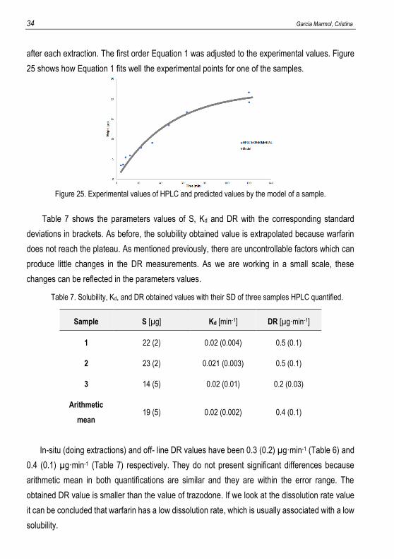
after each extraction. The first order Equation 1 was adjusted to the experimental values. Figure

25 shows how Equation 1 fits well the experimental points for one of the samples.

Figure 25. Experimental values of HPLC and predicted values by the model of a sample.

Table 7 shows the parameters values of S, Kd and DR with the corresponding standard

deviations in brackets. As before, the solubility obtained value is extrapolated because warfarin

does not reach the plateau. As mentioned previously, there are uncontrollable factors which can

produce little changes in the DR measurements. As we are working in a small scale, these

changes can be reflected in the parameters values.

Table 7. Solubility, Kd, and DR obtained values with their SD of three samples HPLC quantified.

In-situ (doing extractions) and off- line DR values have been 0.3 (0.2) µg·min-1 (Table 6) and

0.4 (0.1) µg·min-1 (Table 7) respectively. They do not present significant differences because

arithmetic mean in both quantifications are similar and they are within the error range. The

obtained DR value is smaller than the value of trazodone. If we look at the dissolution rate value

it can be concluded that warfarin has a low dissolution rate, which is usually associated with a low

solubility.


1 22 (2) 0.02 (0.004) 0.5 (0.1)

2 23 (2) 0.021 (0.003) 0.5 (0.1)

3 14 (5) 0.02 (0.01) 0.2 (0.03)

Arithmetic

mean 19 (5) 0.02 (0.002) 0.4 (0.1)


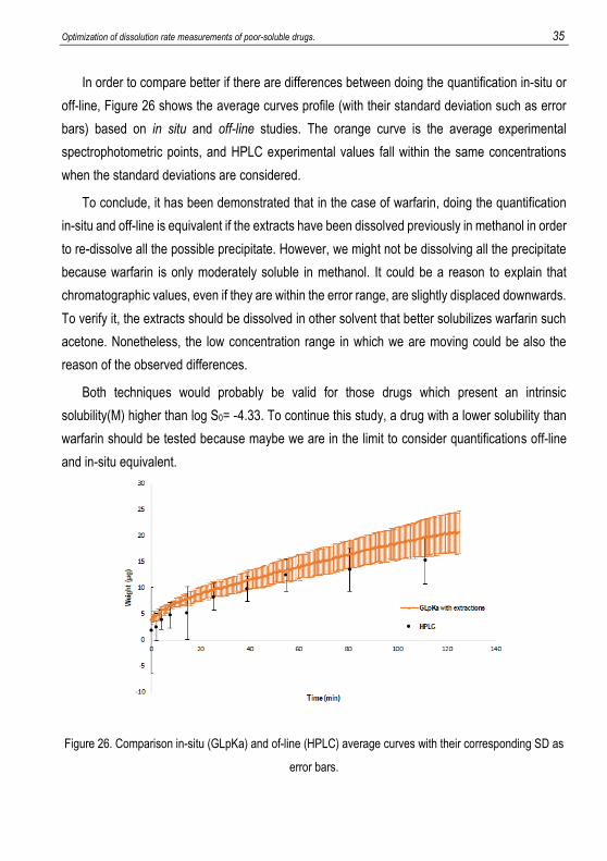
In order to compare better if there are differences between doing the quantification in-situ or

off-line, Figure 26 shows the average curves profile (with their standard deviation such as error

bars) based on in situ and off-line studies. The orange curve is the average experimental

spectrophotometric points, and HPLC experimental values fall within the same concentrations

when the standard deviations are considered.

To conclude, it has been demonstrated that in the case of warfarin, doing the quantification

in-situ and off-line is equivalent if the extracts have been dissolved previously in methanol in order

to re-dissolve all the possible precipitate. However, we might not be dissolving all the precipitate

because warfarin is only moderately soluble in methanol. It could be a reason to explain that

chromatographic values, even if they are within the error range, are slightly displaced downwards.

To verify it, the extracts should be dissolved in other solvent that better solubilizes warfarin such

acetone. Nonetheless, the low concentration range in which we are moving could be also the

reason of the observed differences.

Both techniques would probably be valid for those drugs which present an intrinsic

solubility(M) higher than log S0= -4.33. To continue this study, a drug with a lower solubility than

warfarin should be tested because maybe we are in the limit to consider quantifications off-line

and in-situ equivalent.

Figure 26. Comparison in-situ (GLpKa) and of-line (HPLC) average curves with their corresponding SD as

error bars.


10. CONCLUSIONS

The fact of extracting 10 samples of 50 µL at different times for trazodone and warfarin, does

not significantly affect the dissolution rate profile obtained through the GI dissolution method. In

both cases, the calculated DR parameter (doing extractions and without doing it) was within the

tolerance range, proving that the results obtained with miniaturized are not different when sample

extraction is performed.

The study off-line by HPLC of trazodone’s dissolution rate does not differ significantly from in

situ-study by GI dissolution method in a low volume. However, warfarin has a lower solubility and

differences are observed between the two profiles. The dilution of the extracts with a compatible

solvent increases the concentrations obtained by HPLC, making them equivalent to the ones

determined spectrophotometrically. This indicates that poor-water solubility of warfarin can limit

the quantification off-line by HPLC if a cosolvent is not used.

A dissolution rate study of drug with a higher solubility than warfarin and lower than trazodone

should be performed in order to determine the solubility value from which off-line study cannot be

performed without using a cosolvent. The study of a drug with lower solubility than warfarin should

also be done in order to determine the solubility value which limits completely the quantification

off-line by HPLC (even dissolving extracts in a cosolvent).


11. REFERENCES AND NOTES 1. Shoghi, E., Fuguet, E., Bosch, E. & Ràfols, C. Solubility-pH profiles of some acidic, basic and

amphoteric drugs. Eur. J. Pharm. Sci. 48, 291–300 (2013). 2. Lennernäs, H. & Abrahamsson, B. The use of biopharmaceutic classification of drugs in drug

discovery and development: current status and future extension. J. Pharm. Pharmacol. 57, 273–285 (2005).

3. Pfannkuch, F., Rettig, H. & Stahl, P. H. Biological effects of the drug salt form. in Handbook of Pharmaceutical Salts, Properties, Selection and Use (eds. Stahl, P. H. & Wermuth, C. G.) 117–134 (2002).

4. Pudipeddi, M., Serajuddin, A. T. M., Grant, D. J. W. & Stahl, P. H. Solubility and Dissolution of Weak Acids, Bases, and Salts. in Handbook of Pharmaceutical Salts: Properties, Selection and Use (eds. Stahl, P. H. & Wermuth, C. G.) 19–39 (2002).

5. Dhanapal, R. & Ratna, J. V. Pharmacokinetics and toxicokinetics-A review. Int. J. Innov. Drug Discov. 2, 89–97 (2012).

6. Van de Waterbeemd, H. & Testa, B. The Why and How of Absorption, Distribution, Metabolism, Excretion, and Toxicity Research. Comprehensive Medicinal Chemistry II (Elsevier Inc., 2007).

7. Dressman, J. ., Thelen, K. & Jantratid, E. Towards quantitative prediction of oral drug absorption. Clin. Pharmacokinet 47, 655–667 (2008).

8. Avdeef, A. & Tsinman, O. Miniaturized rotating disk intrinsic dissolution rate measurement: effects of buffer capacity in comparisons to traditional wood’s apparatus. Pharm. Res. 25, 2613–2627 (2008).

9. Bergström, C. A. S. et al. Biorelevant intrinsic dissolution profiling in early drug development: Fundamental, methodological, and industrial aspects. Eur. J. Pharm. Biopharm. 139, 101–114 (2019).

10. Stegemann, S., Leveiller, F., Franchi, D., de Jong, H. & Lindén, H. When poor solubility becomes an issue: From early stage to proof of concept. Eur. J. Pharm. Sci. 31, 249–261 (2007).

11. Kaur, N., Narang, A. & Bansal, A. K. Use of biorelevant dissolution and PBPK modeling to predict oral drug absorption. Eur. J. Pharm. Biopharm. 129, 222–246 (2018).

12. Pobudkowska, A. & DomańSka, U. Study of pH-dependent drugs solubility in water. Chem. Ind. Chem. Eng. Q. 20, 115–126 (2014).

13. Issa, M. G. & Ferraz, H. G. Intrinsic dissolution as a tool for evaluating drug solubility in accordance with the biopharmaceutics classification system. Dissolution Technol. 18, 6–13 (2011).

14. Gravestock, T. et al. The ‘gI dissolution’ method: A low volume, in vitro apparatus for assessing the dissolution/precipitation behaviour of an active pharmaceutical ingredient under biorelevant conditions. Anal. Methods 3, 560–567 (2011).

15. Sasaki, K., Suzuki, H. & Nakawa, H. Physicochemical characterization of trazodone hydrochloride tetrahydrate. Pharm. Res. 41, 325–328 (1993).

16. Kuruvilla, M. & Gurk-Turner, C. A review of warfarin dosing and monitoring. Proc (Bayl Univ Med Cent) 14, 305–306 (2001).


12. ACRONYMS

ADME Absorption, Distribution, Metabolism and Excretion

API Active Pharmaceutical Ingredient

BCS Biopharmaceutics Classification System

DMSO Dimethyl sulfoxide

D-PAS Dip Probe Absorption Spectroscopy

DR Dissolution Rate

GI Gastrointestinal

GIT Gastrointestinal Tract

HPLC High Performance Liquid Chromatography

IDR Intrinsic Dissolution Rate

ISA water Ionic Strength Adjusted water

MEC Molar Extinction Coefficient

MeOH Methanol

SD Standard Deviation

USP United States Pharmacopeia

UV Ultraviolet


APPENDICES


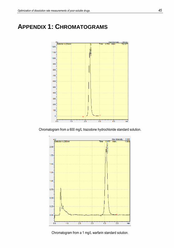
APPENDIX 1: CHROMATOGRAMS

Chromatogram from a 600 mg/L trazodone hydrochloride standard solution.

Chromatogram from a 1 mg/L warfarin standard solution.


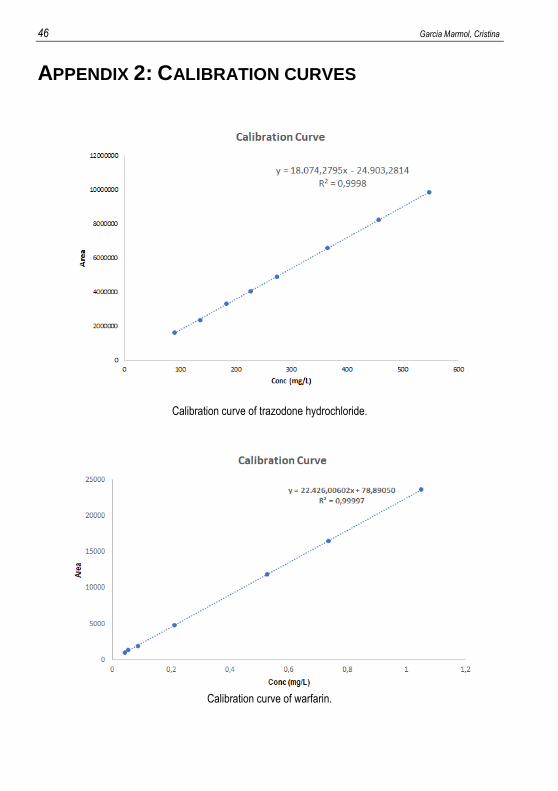
APPENDIX 2: CALIBRATION CURVES

Calibration curve of trazodone hydrochloride.

Calibration curve of warfarin.

Treball Final de Grau - Universitat de Barcelona

Documents

Transcript of Treball Final de Grau - Universitat de Barcelona