


Idiomas
Páginas
Jurídico


BONN-TH-2013-21
Landscaping with fluxes and the E8 Yukawa Point in F-theory
Nana Cabo Bizeta,b 1, Albrecht Klemmc 2 Daniel Vieira Lopesd 3,
a Departamento de Fısica, Division de Ciencias e Ingenierıas, Campus Leon,
Universidad de Guanajuato,Loma del Bosque 103, CP 37150, Leon, Guanajuato, Mexico
b Centro de Aplicaciones Tecnologicas y Desarrollo Nuclear
Calle 30 # 502 e/5ta y 7ma Avenida 11400, Playa, La Habana, Cuba.
c Bethe Center for Theoretical Physics, Universitat Bonn, Nussallee 12, D-53115 Bonn
d CIFMC - Universidade de Brasılia,
Campus Universitario Darcy Ribeiro, Brasılia - CEP 0910-900
ABSTRACT
Integrality in the Hodge theory of Calabi-Yau fourfolds is essential to find the vacuum structure and
the anomaly cancellation mechanism of four dimensional F-theory compactifications. We use the
Griffiths-Frobenius geometry and homological mirror symmetry to fix the integral monodromy basis
in the primitive horizontal subspace of Calabi-Yau fourfolds. The Gamma class and supersymmetric
localization calculations in the 2d gauged linear sigma model on the hemisphere are used to check
and extend this method. The result allows us to study the superpotential and the Weil-Petersson
metric and an associated tt* structure over the full complex moduli space of compact fourfolds for
the first time. We show that integral fluxes can drive the theory to N=1 supersymmetric vacua
at orbifold points and argue that fluxes can be chosen that fix the complex moduli of F-theory
compactifications at gauge enhancements including such with U(1) factors. Given the mechanism
it is natural to start with the most generic complex structure families of elliptic Calabi-Yau 4-fold
fibrations over a given base. We classify these families in toric ambient spaces and among them the
ones with heterotic duals. The method also applies to the creating of matter and Yukawa structures
in F-theory. We construct two SU(5) models in F-theory with a Yukawa point that have a point
on the base with an E8-type singularity on the fiber and explore their embeddings in the global
models. The explicit resolution of the singularity introduce a higher dimensional fiber and leads to
novel features.
May 1, 2014
[email protected]@[email protected]
arX
iv:1
404.
7645
v1 [
hep-
th]
30
Apr
201
4

1 Introduction
The exceptional gauge groups that can arise in F-theory provide an attractive framework for con-
structing GUT models with promising phenomenological properties. This is a common feature with
the heterotic string, where the E8 ×E8 gauge group in 10d is one of two ways to fulfill worldsheet
modularity as well as anomaly cancellation in supergravity. The worldsheet conformal field theory
description of the heterotic string gives a computational framework to make quantitative predic-
tions at least in a region of the coupling space. While this is absent in F-theory important moduli
dependent terms of the N = 1 effective action from F-theory are governed by holomorphic quanti-
ties such as the flux superpotential and the gauge kinetic terms, which are exactly computable using
the variation of the mixed Hodge structures and are technically obtained by a Griffiths residuum
calculation on the F-theory manifold or its mirror. This is particularly effective for fourfolds M
where H3(M) is usually small or zero [1] and the only relevant data are G4 fluxes on H4(M).
F-theory phenomenology is related to singular fourfolds, typically with a singular elliptic fibre, and
there are two useful ways to learn about the structure of the singularity either by analyzing the
homology of the smooth space after blowing it up or after deforming it in the complex structure
moduli space. The former method is at first glance more effective, but since it is only leading
order in the local parameters it misses the subleading effects that do play an important physical
role. The deformations close to the singularity are described by the deformation of the limiting
mixed Hodge with the corresponding residue integrals. This formalism gives not only amplitudes
such as the superpotential exactly as a period integral, but more fundamentally the exact N = 1
coordinates. The point of view that it is more natural to consider the complex deformations has
appeared in many works, see e.g. [2], and reconciles e.g. the higher codimension singularity analysis
in comparison with the simpler group theory expectation from the heterotic string. Calculation of
local complex residua also organize the corrections to Yukawa couplings with many cancellations
among them, see e.g. [3]. While the strength of F-theory should be in the exact geometrical cal-
culation of the holomorphic terms, there are not many results along this line, simply because it
seems a daunting task to analyze the usually huge numbers of periods on phenomenological inter-
esting fourfolds. However using constraints from the Griffiths-Frobenius structure, which leads to
an analog of special geometry for Calabi-Yau fourfolds, and constraints from homological mirror
symmetry, we solve the problem of reconstructing the periods in an integer monodromy basis from
the topological data. Another reason for the interest in the integral basis is that it allows us to de-
fine the tt∗ structure for fourfolds, which is expected to control non-holomorphic corrections beyond
the Weil-Petersson metric. In order to exemplify the method we calculate first the explicit basis
and the monodromies of the periods over the primitive horizontal subspace in nine one-parameter
families including the sextic in P5 and the intersections of five quadrics in P9 and study the periods
at the degenerate points. For the first time one gets hence the exact information about the N = 1
coordinates the superpotential and the Weil-Petersson metric in the entire complex moduli space
of a Calabi-Yau fourfold. Like the seminal calculation for the quintic in P4, these examples have
1

universal features, which generalize to multimoduli Calabi-Yau fourfolds. In particular they have
beside the large complex structure singularity, the conifold singularity, which is the most generic
singularity, and orbifold singularities, which are the model for smooth geometries with additional
discrete symmetries. Part of the results can be checked using the Γ class and the hemi-sphere par-
tition function obtained recently by Hori and Romo using supersymmetric localization and match
perfectly. These latter formalisms are useful to extend our results to hypersurfaces and complete
intersections in toric ambient spaces with many moduli and to the much more general Calabi-Yau
spaces embedded into Grassmannians and flag-varieties described by non-abelian 2d σ-models.
Of course the above approaches to singularities are related by mirror symmetry and one outcome
of the analysis is that, once the leading order analysis in the A-model resolutions is known, the
structures mentioned above are rigid enough so that the exact expression follow relatively swiftly.
F-theory fourfolds with a realistic rank of the gauge group are within the reach of the techniques,
developed in the paper. Explicite heterotic/F-theory moduli identifications ala Friedman, Morgan
Witten allows to find good N = 1 coordinates, moduli stabilizing superpotentials as well as the
uncorrected scalar metric and the tt∗ structure also for bundle moduli in N = 1 heterotic string
compactifications in the stable degeneration limit.
The main question we address here with these new techniques is whether integer flux super-
potentials stabilize F-theory moduli at phenomenological viable compactifications. Using induced
actions of global symmetries on the complex moduli space and the notation of sub-monodromy
systems we argue that these superpotentials can drive F-theory to the loci in the moduli space with
gauge symmetry enhancements and matter structures including the heterotic string limit. We show
explicitly in section 3.11.1 that further moduli can be stabilized at orbifold points and contrary
to the few known attractor points in threefolds, fourfold orbifold points can be attractors with a
vanishing scalar potential. The notion of sub-monodromy systems is very useful in the degeneration
limit and we can give an exact description of the moduli of the central fibre and the heterotic gauge
bundle in the stable degeneration limit.
The superpotentials that we calculate are linear in the periods, which have by definition modular
properties. The reason is that for the theory to make sense in the deformation family of fourfolds
over the vacuum manifold, they have to transform with integral monodromies that respect the
intersection pairing in homology, which we called Q, or η when represented as matrix. Otherwise
the flux quantization condition and the metric of the scalars would not be uniquely defined. These
transformation properties makes the periods meromorphic modular forms w.r.t. to the discrete
symmetry group Γ generated by the monodromies. The latter are more fundamental, because the
Riemann Hilbert problem is solved in this context, meaning that the monodromies determine the
periods as those meromorphic sections over the complex moduli that have reasonable behaviour at
the boundaries of the moduli space. If non-perturbative effects respect Γ, then the corresponding
superpotential will be modular and hence reconstructable from a very restricted set of meromorphic
2

sections. A striking example of such a non-perturbative superpotential with modular properties
was given in [4] and as we explain in section 5.2.2 it is simply the period on the mirror manifold.
By the same principle F-theory periods encode very valuable information about the non-
perturbative corrections to the perturbative theories that arises in degeneration limits. This implies
for the heterotic string [5][6][7] that small instantons as well as the associated heterotic 5-brane
moduli can be identified and e1/gs effects can be calculated. Moreover the open/closed duality
between the F-theory at genus zero closed string sector and the Type II disk open string string
sector [8][9] that has been computationally established in those non-compact limits, allows [6] to
study D-instanton corrections in orientifold compactifications. The relations between fourfold pe-
riods and type II D5-brane open string superpotentials has been intensively studied [5][10][11][12].
Moreover the fourfold superpotential also captures important aspects of the vacuum structure of
manifolds with SU(3) structure, see e.g. [13].
The paper is divided roughly into two parts and organized as follows: Until section five we
deal with properties of F-theory that are useful to analyze the complex structure moduli, the flat
coordinates and the integral structure on the primitive horizontal subspace, including the modular
properties of the amplitudes. In section 2 we give a conceptual overview over challenges in F-theory
model building on compact Calabi-Yau manifolds. The geometrization of the Type IIB axio-dilaton
in elliptic fibrations, its dependence on the moduli of the fourfold as well as a short discussion of
the non-perturbative limits can be found in 3.1, while the basic properties of its compactification
are spelled out in section 3.2. The section 3.3 gives those topological and geometrical properties
of fourfolds in particular its Hodge structure and its integer structures that are used throughout
the paper. The construction of Batyrev and Borisov is set up in section 3.4.1 together with a
discussion of implementation of twisted fibration structures in section 3.4.2. Beside the aspect
of mirror symmetry that turns out to be essential for F-theory, other main advantages of the
construction is that it gives a good model of the moduli spaceMcs described in section 3.5 and the
points of maximal unipotent monodromy, see section 3.5.1. Using the model of the moduli space
developed in section 3.5 we study the induced group actions on it in section 3.6 and give a local
account of the behaviour of the periods near orbifold points. In preparation of the discussion of the
sub-monodromy systems that extend this local picture, we discuss in section 3.6.2 the transitions
that are described geometrically by embedding polyhedra into each other. In section 3.7 we define
the notion of the sub-monodromy system using the Picard-Fuchs ideal and its D-module and argue
that the embedding of polyhedra defines sub-modromy systems on the locus S ⊂Mcs. We discuss
the relevance of the degenerations of Calabi-Yau manifolds and its description using limiting mixed
Hodge structure to the sub-monodromy systems, the fixing of an integral basis and the approach of
gluing amplitudes from degenerate components in stable limits. We correct some statements in the
physics literature concerning the application of Schmids nilpotent orbit approximation, which is
incompatible with the Γ-classes. In section 3.8 we review the terms that are calculable exactly and
approximatively from the holomorphic– and the real geometrical structures of 4-folds respectively.
3

3.9 — 3.11 are the main sections of the first part where we fix the integral monodromy basis
and draw conclusions for the N = 1 vacua structure in F-theory. In section 3.9.1 we use the
Frobenius structure, the Griffiths transversality and the real structure of the Calabi-Yau n-folds
to define the real Griffiths-Frobenius structure, which in particular includes special geometry and
the tt∗ structure. It remains incompletely specified until we find the integral basis. We review this
procedure for 3-fold stressing the general aspects in 3.9.2. In section 3.9.3 we find the integral basis
for nine fourfolds and all its monodromy- and connections matrices as well as the flat coordinates
throughout Mcs by explicit calculation. In section 3.10 we relate the calculation to homological
mirror symmetry and check the occurrence on the Γ class at the maximal unipotent degeneration.
In section 3.10.2 we check and extend the results of 3.9.3 using the hemisphere partition function
of Hori and Romo, with boundary data specified by Chan-Paton factors and matrix factorizations.
For complete intersection and hypersurfaces in toric varieties one gets a rational K-theory basis of
twisted line bundles on the mirror, whose intersection is simply defined by the Chern character map
and the Hirzebruch-Riemann-Roch index theorem. Continuation of Barnes integral representation
of the HPF relates the rational basis to our integral basis and the intersection forms for the two
basis match perfectly. We also generalize the HPF to local CY and relate the HPF to the Picard-
Fuchs ideal. We discuss the general features for minimizing the superpotential in section 3.11. In
section 3.11.1 we use the integral basis to establish that the superpotential drives the moduli to
the orbifold point with a vanishing scalar potential. We analyze the superpotential at the most
generic singularity, the node in section 3.11.2, which has very different features depending on the
dimension n of the CY mod 4. Given the superpotential in the integral basis we come back to the
sub-monodromy system in section 3.11.3 and formulate a general conjecture based on the examples
discussed before. In section 4 we classify the clean sheet models starting with the heterotic basis
in section 4.1 and a small statistic of the topological data of the more general 4319 toric almost
Fano basis in section 4.2 and the generic global fibres in the complete intersection class 4.3. For
the embeddings of polyhedra we get a sub-monodromy system and a superpotential that restricts
the moduli to subloci S . This will be used in section 5 to construct first non-abelian gauge groups
in the models discussed in section 4 by restricting polyhedra to reflexive subpolyhedra. We start in
sections 5.2 and 5.2.1 by enforcing the stable degeneration limit and identify the sub-monodromy
system that governs the moduli space, metric and flat coordinates of the central fibre as well as
of the one that governs the same data on the heterotic gauge bundle moduli in section 5.2.2. We
explain the occurrence of the modularity in the partition functions for the gauge degree of freedom,
which can be interpreted in terms of [p, q]-strings. In section 5.3 we extend that to models with
additional U(1)′s. In particular we use Nagells algorithm to bring the corresponding normal forms
of the fibres into Weierstrass form and relate the gauge groups to vanishing of the coefficients of
the normal forms for the E7 fibre and the E6 fibre in sections 5.3.1 and 5.3.2 respectively. In
section 5.3.3 we construct series of Calabi-Yau n-folds that go back to an observation of Pinkham
regarding the realization of Arnolds strange dualities in K3’s. The cases hold the current records
for the topological data for Calabi-Yau n-folds w.r.t to Euler number and number of complex
4

deformations for all n. As such they are another logical starting point for the landscaping with
fluxes, but with an E6, E7, E8, . . . gauge group unhiggsable by complex structure deformations.
The second part of the paper is devoted to study the F-theory models with SU(5) gauge group
and codimension 3 singularities (Yukawa points) expected to be of E8 type i.e. on the studied locus
the vanishing order of the coefficients in the Weierstrass form describing the elliptically fibered
fourfold is the one of a codimension 1 E8. In the work of Esole and Yau [14] small resolutions of
SU(5) GUT models were studied, to obtain singularities with codimension higher than 1 which
resolutions differ from the expectations obtained by following Kodaira classification. The study
realized by Marsano and Schafer-Nameki [15] considers the codimension 3 E6 kind singularity, to
show that even if after resolving a different structure arises, the physics is as expected. Motivated
by the fact that the Yukawa couplings giving rise to the neutrino mixing matrix were obtained by
Heckman, Tavanfar and Vafa [16] to arise from an E8 singularity, and by the previously mentioned
works we explore the resolution of codimension 3 singularities expected to be of E8 type, to find
results that differ from the expectations, see sec 7.4. In section 6 we present those models. Section
6.1 is devoted to explore the realization of the codimension 3 E8 singularities in the global toric
models constructed in sec 5. In section 6.2 we describe the models with SU(5) gauge group
which carry a codimension 1 SU(5) singularity, and its resolution. Those models present further
singularities in higher codimension, and in section 6.3 we propose a way to study the expected
codimension 3 E8 enhancement based on the F-theory/Heterotic duality via the spectral cover
construction and the group decomposition E8 → SU(5) × SU(5)⊥. We choose two different local
models which give an E8 type vanishing order for the coefficients in the Weierstrass form of the
elliptic fibration. The first of those is Case 1, which contains matter representations 5 and 10. This
model is studied in section 7. In section 7.1 we perform its resolution, by blowing-up ten times
with P1 and P2’s in the ambient space. In section 7.2 we describe the codimension 1 locus obtained
after the resolution. In section 7.3 we describe the codimension 2 locus, the matter curves 10 and
5 obtained in the resolution with its respective gauge group charges and its weights. Section 7.4
is devoted to the analysis of the codimension 3 locus, which turns out to differ from the expected
E8. In the appendix B.1 we give the details of this blowup, and in appendix C we describe how the
charges are computed. In section 8 we study the resolution of an SU(5) model with a codimension
3 E8 singularity in which there is a certain symmetry among the two basis coordinates which
vanishing (above the SU(5) locus) gives the singularity locus, we denote this Case 2. We follow
identical steps as for Case 1, and in sec 8.1 we perform the resolution by eight blow-ups, in sec 8.2,
8.3 and 8.4 we describe the blow-up obtained codimension 1, 2 and 3 locus respectively. In sec 8.5
we comment on the implications of the symmetry present in Case 2. Appendix B.2 contains the
details of the Case 2 resolutions. Finally we give our conclusions in section 9.
5

2 Elements of F-theory phenomenology
In F-theory [17] the relevant data are described in terms of the geometry of a Calabi-Yau n-fold
Mn, elliptically fibred EF → Bn−1 over a base Bn−1 and a choice of G fluxes. By definition Mn has
an unique holomorphic (n, 0)-form Ω and an (1, 1) Kahler form J . For compactifications to eight
dimensions M2 is hence an elliptic K3 manifold, B1 = P1 and F-theory, or equivalently Type IIB
on B1 with varying axion C0 and dilaton φ background encoded in the complex structure τ of EFas τ = C0 + ie−φ, with eφ = gIIB the type IIB string coupling, yields a more general 8d theory
then the E8 × E8 heterotic string4 on T 2. In fact it contains the latter in the stable degeneration
limit, in which the K3 decomposes into two half K3’s, i.e. rational elliptic surfaces describable
as the 9-fold blow of P2 called dP9, with the heterotic torus T 2 as the central fibre. In short the
degenerate geometry is given by limhetK3 = dP9 ∪T 2 dP9.
Lower dimensional F-theory/heterotic duals can be obtained by fibering the dual 8d compact-
ification data K3/(T2 + gauge bundles) over a common base Bn−2, i.e. in compactifications to
4d B3 becomes a rational fibration P1 → B2 over a basis B2. The F-theory K3 is realized as an
elliptic fibration over the above P1, so that M4 becomes an elliptic fibration over B3 as well as a
K3 fibration over B2, while the heterotic Calabi-Yau 3-fold Z3 is an elliptic fibration Ehet → B2.
This construction still has a heterotic limit limhetM4 = P4 ∪Z3 P4, where P4 has the fibration
structure of M4 with K3 replaced by the half K3, and the matching of the compactification data
on both sides is well understood [23]. This includes a dictionary between heterotic moduli and the
moduli of Mn. In particular the bundle moduli are mapped to the complex structure moduli of Mn
and the choice of the intermediate Jacobian JMn = H3(Mn,R)/H3(Mn,Z). For n = 4 one always
has H3,0(M4) = 0 and frequently H2,1(M4) = 0 hence H3(M4) = 0, so the intermediate Jacobian
becomes either trivial or an abelian variety5. This very geometrical description of F-theory in
terms of the fourfold geometry allows to determine the holomorphic terms in the four dimensional
N = 1 effective action. The easiest example is the superpotential, which makes (heterotic) moduli
stabilization possible6. The latter is determined by the fourfold periods and includes in particular
non-perturbative corrections to the heterotic string and the orientifold theories that arise in the
limits of F-theory and have been identified in [5]-[13] .
Using the M-theory/F-theory lift, it was explained in [24] that a (half) integer quantized [x] =
[G4− c2[M4]/2] ∈ H4(M4,Z), primitive (J ∧G4 = 0) flux G4 = dC3 in H4(M4,Z), which fulfills the
tadpole condition (3.15) and is compatible with the fibration structure, leads to a superpotential
Wcs(a) =
∫M4
Ω(a) ∧ G4
2π, (2.1)
4The heterotic SO(32) [18, 19] and the CHL [20, 21, 22] string can be accommodated in the F-theory geometry.5In the latter case one can twist it [23] by a G4 flux in H2,2(M4), so that this part of the moduli is described by
Deligne cohomology of M4.6Unfortunately the adiabatic argument requires the elliptic fibration structure and large volumes on the heterotic
side, which prevents a direct F-theory description of heterotic orbifolds.
6

which fixes the otherwise unobstructed complex structure moduli a of M4 so that G4 is of Hodge
type (2, 2), which implies that it is self-dual. For arbitrary G4, i.e. if the primitivity condition
J ∧ G4 = 0 does not hold, one can view it as a condition enforced on the Kahler moduli t by
minimizing a superpotential
Wks(t) =
∫M4
J2(t) ∧ G4
4π. (2.2)
Minimization of (2.1,2.2) encompasses geometric as well as the bundle moduli of the heterotic
string. The splitting of the superpotential and more importantly the Kahler potential into the
two types of chiral N = 1 fields is an approximation, which will be in general invalidated by
non-perturbative effects. Nevertheless because of the positivity of the individual contributions to
the F -term superpotential the minimization of the terms coming (2.1) and (2.2) can reveal the
structure of the vacuum manifold even in the presence of certain mixings. An example for a non-
perturbative superpotential that gives additional constraints on the Kahler moduli that depend
mildly on a is the non-perturbative superpotential that comes from the M5 brane wrapping a D
in M4, which has to have Dirac index χD(G) = h00 − h10 − h30 + n(G4) = 1 with n(0) = h2,0
and n(G4) ≤ h2,0 [25, 4, 26]. This superpotential can be mapped to F-theory for vertical divisors
and has been identified with the supersymmetry breaking effect due to gluino condensation [27].
This can eventually provide a mechanism for the KKLT uplift. Even if the splitting is only mildly
broken, the constraints from (2.1) that depend on the primitive part of G4 and the one of (2.2) that
depend on the non-primitive part of G4 can in general not be separated, because an (half) integer
basis of Hn(Mn,Z) correlates elements in Hnprim(Mn) and Hn
notprim(Mn) with rational coefficients
as discussed in section 3.3.
While (2.1) can stabilize complex moduli, one of the most challenging problems in F-theory
is to find out whether there are G4 fluxes that drive the moduli to the degenerations that one
needs to create those structures suitable for phenomenology, in particular the heterotic string
and more general gauge symmetry enhancements at codimension one, matter curves and Yukawa
points at higher codimension in the base e.t.c. An equally important and challenging problem is
to fix the other moduli without creating unwanted further structures. For illustration consider the
universal K3, with stringy moduli space MK3 = O(4, 20,Z)\O(4, 20)/(O(4)×O(20)). While type
II compactifications on this geometry have generically no gauge symmetry enhancement, one could
realize the K3 in many ways algebraically, e.g. as section of the anticanonical bundle in those toric
varieties P∆3 , which correspond to the 4319 3d reflexive polyhedra. The corresponding complex
families frequently have a rank r gauge group, because they live in codimension r in the K3 moduli
space specified by the Noether-Lefschetz divisors 7. However picking the algebraic representation
of the K3 in P∆3 is ad hoc and one wishes to have a physical mechanism, e.g. a potential that
starting for the universal K3 explains, why the physical model lives on a set of measure zero in the
7The Noether-Lefschetz divisor of the fibre is preserved in algebraic realizations of K3 fibred Calabi-Yau manifolds,a fact that was recently used to prove the Yau-Zaslow conjecture relating the elliptic genus of the heterotic stringsto IIB counting functions of higher genus curves in K3 using modular forms [28].
7

moduli space. For three or four dimensional Calabi-Yau spaces there is no universal moduli space
in the sense of MK3, but there are good indications that there are huge connected components
of universal moduli spaces, which can be connected by transitions. E.g. one can argue that all
Calabi-Yau 3-folds realized as anticanonical bundle in P∆4 are connected [29] in one moduli space.
For fourfolds from the purely geometric point of view this is likely to hold for embeddings of r
transversal polynomial constraints in in P∆5+r , which we review in sect. 3.4.1. However N = 1
vacua require in general fluxes that have to change a least in certain transitions [1, 30] to fulfill the
tadpole cancellation condition. Therefore one can have discrete connected components.
The most sensible way to address the flux problem is hence to start within a generic member of
a family Calabi-Yau of manifolds in a particular component with no gauge group. Its convenient
to fix the base B3 of the family, since transitions by blow ups in the base of a fourfold were studied
already in [1] and first classify all elliptic toric hypersurface Calabi-Yau manifolds, which have no
gauge group and no tensionless strings. These we call the clean sheet fibrations. We first classify
all those basis, which are P1 fibrations over a toric bases B2 in section 4.1. The interest in these
models is that they have heterotic duals with completely higgsed gauge bundle over the same basis
B2. These models are all members of a class geometries, for which the basis of the elliptic fibration
is a toric projective space P∆3 associated to the before mentioned 4319 three dimensional reflexive
polyhedra. The corresponding classification of properties of the clean sheet models is done in
section 4.2. We then search for fluxes, which can drive the family to gauge theory limits and create
further structures at higher codimension. We call this process landscaping by fluxes. To implement
it concretely it we use Batyrev’s approach to mirror symmetry, which constructs mirror pairs of
hypersurfaces and complete intersections in toric ambient spaces. The reason for staying in this
manifestly mirror symmetric class is that structures implied by homological mirror symmetry are
very useful to get a basis for Hnprim(Mn) and the periods. The bulk of the investigation focusses
on the question, how to pick the part of G4 in Hnprim(Mn) that does the landscaping to the desired
configurations in the complex moduli space. The conditions to find an N = 1 supersymmetric flux
vacuum are reviewed in sect. 3.11. On an N = 2 Calabi-Yau background with fluxes they are
equivalent to find solutions to the attractor equations for supersymmetric black holes [31]. The
study of the minima of flux superpotentials requires to find special points in the period domain of
Calabi-Yau spaces a problem related in a very fascinating way to arithmetic and number theory [32].
In the second part of the paper we study a degeneration of the complex structure, which
is phenomenologically motivated. SU(5) GUT model building with D branes and orientifold-
branes has perturbatively no 5Hu10 10 coupling, which would give the required order 1 Yukawa
coupling for the top quark, a fact which is remedied in F theory when one starts with an Ek≥6
symmetry enhancement in complex codimension three over the base. It has been further argued
that a hierarchy in the Cabibbo-Kobayashi-Maskawa (CKM) quark mixing matrix leads naturally
to k ≥ 7, while the corresponding hierarchy in Pontecorvo-Maki-Nakagawa-Sakata (PMNS) matrix
for the lepton sector and an phenomenological acceptable µ terms favors k = 8[33, 34, 16].
8

Gauge symmetry enhancement in the 4d part of the 7-brane with gauge group G occurs at
divisors Dg in B3 wrapped by the 7-brane — for the decoupling scenario chosen to be the above B2
— over which the elliptic fibre degenerates to ECg : A collection of vanishing P1, whose intersection
is given by the negative of Cartan-matrix Cg of the corresponding affine Lie algebra g associated
to G. This yields an elliptic singularity of the Kodaira type labelled by g (also the ˆ is usually
dropped). These singularities can be classified on complex co-dimension one loci over the base by
the vanishing order of the Weierstrass data 8 of the elliptic fibration M4 at Dg as made explicit
below. In order to capture in addition the monodromy data for elliptic singularities in codimension
2 in the base, which acts as an outer automorphism on the P1 in ECg , which correspond to the
simple roots, to yield non-simply laced Lie groups, one needs information encoded, for simple fibre
types in the Tate form or analogous normal forms of the elliptic fibre.
The matter spectrum and its representations is determined from enhancements of the elliptic
fibre singularity ECg → EC′′ over a co-dimension two (matter)-curve ΣM = Dg∩Dg′ , or ΣM ⊂ Dg if
Dg is not smooth, in the base. The chiral spectrum is determined by the gauge symmetry breaking
G4-flux Gb4, in particular the chiral index is given by
χ+ − χ− =
∫ΣM
i∗(Gb4) . (2.3)
The tree level Yukawa couplings are related to a further enhancement of the elliptic fibre ECg′′ →EC′′′ over a co-dimension three (Yukawa)-point P = Dg ∩Dg′ ∩Dg′′′ .
Commonly it was assumed in the phenomenological analysis of F-theory that C ′′ and C ′′′ are
given by the group theory expectations and that this can be confirmed by the Tate data of M4.
However a direct resolution of the singularities at the claimed codimension two and three where
the enhancements to the E6 exceptional group was claimed shows a picture which contradicts these
expectations [14].
We analyze this mismatch and the physical consequences of the actual resolution for the E8
point. First we discuss the SU(5) model, which embedded into F-theory has attractive phenomeno-
logical features. We then describe the complex structure to obtain the E8 point and proceed with
a detailed analysis of the resolutions process in increasing codimension.
In such general case, the singularities enhancements can be resolved via small resolutions as
done in [14] and further explored in [15].
8There are some cases in which one needs as an extra condition the factorization of a polynomial to cause thesingularity, those are the split cases [35].
9

3 F-theory and Calabi-Yau n-fold geometry
In this section we review the general construction of F-theory and prepare for the compactifications
with gauge symmetry enhancements over divisors in the base using Kodaira’s and Tate’s algorithms.
We then argue that this gauge symmetry enhancement is induced by the F -terms of G4 fluxes and
describe the realization of that mechanism for toric Calabi-Yau manifolds using general arguments
about the symmetries in the complex moduli space, the constraints of Griffiths transversality, the
Frobenius structure and some general properties of the period map.
3.1 The F-theory ‘map‘ and its perturbative limits
Every family of elliptic curves can be written in the Weierstrass form, which reads in affine complex
coordinates x, y as
y2 − 4x3 + fx+ g = 0, (3.1)
where ∆ = f3 − 27g2 is the discriminant of the curve. The complex structure of the elliptic curve
τ is related to f and g by
j(q) = 123 f3
∆, (3.2)
where q = exp(2πiτ) and j(q) = (12E4)3/(E34 − E2
6) = 1q + 744 + 196884q + . . .. For k ∈ 2N+
Ek =1
2ζ(k)
∑n,m∈Z
(n,m)6=(0,0)
1
(mτ + n)k= 1 +
(2πi)k
(k − 1)!ζ(k)
∞∑n=1
σk−1(n)qn , (3.3)
are normalized (and regularized by the second equal sign for k = 2) Eisenstein series, with σk(n)
the sum of the k-th power of the positive divisors of n and ζ(k) =∑
r≥0 1/rk, which equals
−(2πi)kBk/(2k(k − 1)!) for k ∈ 2N+, with∑∞
k=0Bkxk/k! := x/(ex − 1).
For a family of elliptic curves f and g depend on one complex modulus, but in a fibration
they depend on the coordinates u of the base Bn−1 and of the complex moduli a of Mn, so that
(3.2) yields a ‘map‘ from (u,a) to the axio-dilaton τ . The complex moduli of M4, typically in
the order of thousands for compact fourfolds [1] describe the complex moduli of Bn−1, but mostly
the profile of j over Bn−1. Like j is compactified in P1 with special points, the full complex
moduli space parametrized by a ∈ Mcs is compact with normal crossing divisors. Eq. (3.2)
defines the ‘map‘ up to a PSL(2,Z) action on τ , as j(τ) is invariant under τ 7→ τγ = aτ+bcτ+d with
γ =(
a bc d
)∈ SL(2,Z), which follows from the definition of j and the first identity in (3.3) that
obviously implies Ek(τγ) = (cτ + d)kEk(τ) for9 k > 2. This corresponds to an ambiguity in the
choice of a type IIB duality frame. One cannot chose globally a weak coupling duality frame, as
τ undergoes monodromies over paths in Bn−1 around ∆, which generate a finite index subgroup
9For k = 2 the second equality is taken as a regularization description for the sum in the first terms, which breaksthe modular transformations and lead to almost modular forms.
10
ΓM ∈ PSL(2,Z), which does not preserve the weak coupling choice τ ∼ i∞ (1/j ∼ q = 0). This
means that F-theory necessarily contains non-perturbative physics.
The closest one gets to a perturbative description is to consider limits in a, referred to as weak
coupling limits, where the profile of j is such that 1/j ∼ 0 almost everywhere over Bn−1. Depending
on the global limiting profile, near the points where this fails, some of the complex structure moduli
a can be understood as moduli of seven branes in orientifolds [36] or as the moduli of the heterotic
string [23]. By analyzing these perturbative limits and identifying carefully the map between the
F-theory parameters and the parameters of the perturbative theory one can learn about the non-
perturbative corrections. For example by distinguishing between the brane and the bulk moduli
one can learn about the disk-instanton corrections of the brane [5][10][11][12] Non-perturbative
corrections in the heterotic string have been identified in [6][7]. By a tentative identification of the
dilaton, D-Instanton corrections can be isolated [6].
Picking the correct field basis and the integer flux basis is essential for the anomaly cancellation
mechanisms in the perturbative theory in four dimension. An interesting example is the central
charge formula for the D-branes (3.124) that directly reflects the properties of the integrals basis.
It is almost the one that governs the anomaly inflow for the flat branes [37], but the replacement
of the square root of the A-roof genus by the Γ class induces corrections that affect the anomaly
inflow mechanism in perturbative limits of global F-theory compactifications. Many of the four
dimensional conditions will be traced back to (3.14) and one would expect all local limits fulfilling
the global tadpole cancellation to be consistent four dimensional theories. That the integral basis
is crucial in the analysis can be also seen from the chirality index (2.3) depends on the integrality
of the cohomology of the flux basis and the dual cycles. On the other hand understanding the 4d
and 3d anomaly cancellations mechanism better, give new methods to fix the integral basis and
insights in the geometry of fourfolds.
The map (u,a) to j will have ramifications points, which lead to monodromies acting the
cohomology of the fibre along paths in (u,a) . The Galois group of the map is crucial for the global
fibration structure and the physical spectrum. In particular it determines the number of sections of
the elliptic fibration and the question, which ΓM and which subgroup Γ = PSL(2,Z)/ΓM is realized
in the theory [21, 22].
3.2 Compactifying the Weierstrass model
In compactifying (3.1) over Bn−1 to Mn the triviality of the canonical bundle KMn = 0 requires,
at least for a suitable choice of a birrational model [38, 39],
KBn−1 = −∑
ag[Dg] , (3.4)
where ag > 0 depends on the Kodaira type of the singular fibre given in table A.1.
11

One convenient method to construct compact algebraic Calabi-Yau fourfolds with tunable gauge
theory enhancements is to construct first an ambient space as a fibration of a projective toric variety
P∆F over a projective toric variety Bn−1 = P∆B and as a second step the algebraic Calabi-Yau
manifolds in this ambient space.
A special role in the construction of smooth elliptic fibrations is played by Fano varieties X,
which are smooth projective varieties with ample anticanonical divisor −KX . By Kleinman’s
criterium [40] a divisor is ample if it is in the interior of the cone spanned by the numerically effective
divisors or equivalently its intersection with all numerically effective curves is positive. Physically
it is sensible to include also smooth projective varieties as basis Bn−1 for which −KBn−1 intersects
only semi-positive on the numerically effective curves. This is a generalization of the notion in [23],
where it was used to include the resolution of del Pezzo surfaces with ADE singularities. The
resolution introduce rational −2 curves C as exceptional divisors, for which the adjunction formula
(K + C) · C = 2g − 2 implies K · C = 0. In the 2d toric case these are only Ak singularities
and correspond to the points on the edges of the 2d polytopes in Fig. 1. As in [23] we call the
corresponding varieties almost Fano varieties even though following notion of pseudo ampleness [40]
pseudo Fano might be more appropriate.
If Bn−1 is a toric almost Fano basis in this sense one can construct a smooth elliptic fibration.
This is because [∆] = −12KBn−1 , [f ] = −4KBn−1 and [g] = −6KBn−1 and by the semipositivity
the generic discriminant ∆ vanishes at a divisor D in Bn−1 at most with order one and since [f ]
and [g] can then not vanish both at D one gets according to table A.1 at most an I1 singularity
in codimension one. The existence of the positive support function φ, described in section 3.4.1,
guarantees that the basis Bn−1 = P∆B , where ∆B is reflexive, are toric almost Fano varieties.
One gets different fibre types by constructing the generic smooth fibre as the anticanonical
divisor in a 2d toric almost Fano variety corresponding to a reflexive polyhedron. This leads to
the generic E6, E7 and E8 fibre types and to non-generic cases of En<6 fibre types. En fibres give
rise to models with k = 9−n sections and U(1)k global gauge symmetry. A framework to describe
the compact Calabi-Yau manifolds is again as the anticanonical divisors (or suitable complete
intersections) in toric ambient spaces related to reflexive polyhedra discussed in section 3.4.1.
The corresponding F-theory compactifications have no non-abelian gauge group or equivalently
within a given fibre type the most generic Higgs bundle over the base. Then in further steps one
enforces by specialization the complex structure singular fibres along gauge divisors, the matter
curves and the Yukawa points.
3.3 General global properties of Calabi-Yau fourfolds and flux quantization
In this chapter we discuss general global properties of compact Calabi-Yau manifolds Mn, mainly
for complex dimension n = 4. We refer already to some results of section 4.3, which is devoted to
12
global properties that do depend on the fibration structure.
Let χq =∑dim(Mn)
p=0 (−1)php,q be the arithmetic genera. Then we have from the Hirzebruch-
Riemann-Roch (H-R-R) theorem [41] for B3 a rational surface, i.e. with first arithmetic genus
χ0 = h0,0 = 1, that
1 = χ0 =1
24
∫B3
c1c2 . (3.5)
For a Calabi-Yau fourfold with first arithmetic genus χ0 = h0,0 +h4,0 = 2 the H-R-R theorem gives
2 = χ0 =1
720
∫M4
(3c22 − c4), χ1 =
1
180
∫M4
(3c22 − 31c4), χ2 =
1
120
∫M4
(3c22 + 79c4), (3.6)
which yieldsh2,2 = 2(22 + 2h1,1 + 2h3,1 − h2,1) ,
χ(M4) = 6(8 + h1,1 + h3,1 − h2,1) .(3.7)
I.e. to infer the full Hodge diamond of a fourfold M4, we can use its Euler number and the Hodge
numbers hn−1,1, h1,1. H4(M4) splits into a selfdual (∗α = +α) and an anti-selfdual (∗α = −α)
subspace
H4(M4) = H4+(M4)⊕H4
−(M4), (3.8)
whose signature follows from the Hirzebruch signature theorem [41] as
σ = h4+(M4)− h4
−(M4) =
∫M4
L2 =χ
3+ 32 , (3.9)
where the second L polynomial is L2 = 145(7p2 − p2
1) with the Pontryagin classes p1 = c21 − 2c2
and p2 = c22 − 2c1c3 + 2c4. H4(M4) also splits into an horizontal part generated by ∇|a|a Ωn, see
section 3.8.1, which is primitive J ∧ αprim = 0, and a vertical part generated by Lefschetz SL(2)
action with J as the raising operator [42]. For fixed moduli the dual cycles can be calibrated
symplectically with Re(eiθΩn) or holomorphically with Jn
n! . In addition there can be Cayley cycles
calibrated with 12J
2 + Re(eiθΩn) on fourfolds, see [43] for a review on calibrated geometries. These
structures are exchanged by mirror symmetry. The only vertical part sits in H2,2(M4) = H2,2H (M4)⊕
H2,2V (M4). On the middle dimensional cohomology one has a bilinear form Q : Hn ⊗ Hn → C,
defined by
Q(α, β) =
∫Mn
α ∧ β (3.10)
with the property
Q(Hp,q, Hr,s) = 0 unless p = s and q = r , (3.11)
and for primitive forms in the middle cohomology α ∈ Hp,q the positivity of the real structure
R(α, α) = ip−qQ(α, α) > 0 , (3.12)
13
equips Hn(Mn) with a polarized Hodge structure. For n = 3 or more generally odd all α are
primitive and Q becomes the familiar symplectic pairing 10, while in the n = 4 case one gets the
following signature eigenspaces
H4,0 ⊕ H3,1 ⊕ (H2,2prim, J
2) ⊕ H2,2notprim ⊕ H1,3 ⊕ H0,4
+ − + − − +(3.13)
Here the h1,1 − 1 not primitive (2, 2)-forms J ∧ αnotprim 6= 0 are generated as J ∧H1,1prim [42].
Physically, one has from the equation of motion for the G4-flux on M4
d ∗G4 =1
2G4 ∧G4 − I8(R) +
∑i
δ(8)i Qi2 +
∑i
T 3 ∧ δ(5)i Qi5, (3.14)
which implies (24∫M4
I8(R) = χ(M4)) the global tadpole condition
1
2
∫M4
G4 ∧G4 +NM2 =χ(Mn)
24, (3.15)
where we exclude the M5 branes This can be lifted to F-theory turning the M2- to D3-branes. Of
course consistency requires NM2 = ND3 ∈ Z. Let us summarize some facts:
• i) The second equation in (3.7) implies χ(M4) = 0 mod 6. One finds χ(M4) 6= 0 mod 24 for
roughly a fourth of the Calabi-Yau fourfolds in weighted projective space [1] independently
of the fibration structure. These cases require half integer fluxes.
• ii) One finds that the clean sheet models over almost Fano basis, i.e. without non-abelian
gauge groups, have always χ(M4) = 0 mod 24 and require no fluxes. This follows for the
E6 − E8 fibre type from (3.5,4.18), while for the D5 fibre type one has to invoke in addition
(4.10) for n = 3.
• iii) On the other hand Wu’s formula [x]2 = c2 ∧ [x] mod 2 and the first equation in (3.6)
implies that any flux obeying [x] = [G4 − c2/2] ∈ H4(M4,Z) leads to ND3 ∈ Z [45].
• iv) H4(M4,Z) ∼ H4(M4,Z) is unimodular by the Poincare pairing. Hence if c2 is even,
i.e. c2 = 2y with y ∈ H4(M4,Z), then H4(M4,Z) is an even unimodular lattice. Even
unimodular lattices with trivial signature exist only in dimension d = 0 mod 8. Moreover the
negative eigenvalues in H4(M4,Z) pair with positive ones into hyperbolic rank two lattices
H =
(0 11 0
)[46] and the others form the even selfdual unimodular E8 lattices so that
H4(M4,Z) = H⊕m ⊕ E⊕k8 , (3.16)
10For n = 3 one has (−i, i,−i, i) on (H3,0, H2,1, H1,2, H0,3). This leads the definition ofNΣΛ to make the graviphotonkinetic term in N = 2 supergravity positive, see [44] for a review. For n = 2, i.e. K3 one has from the HST withL1 = 1
3(c21 − 2c2) that σ =
∫K3
L1 = −16 and −1, 1,−1 on (H2,0, Hprim1,1 , H0,2), and H2(K3,Z) = H⊕3 ⊕ E⊕2
8 (−1).
14

with m = (b4 − σ)/2. One corollary for even lattices using (3.9) is that σ = 0 mod 8 so that
χ(Mn) = 0 mod 24 and k = σ/8 [1]. This is true for the clean sheet models. If H4(M4,Z) is
not even, it is diagonalizable w.r.t. to the bilinear form Q over the integers [46].
• v) Using (4.15), Table 3.2 and explicit calculations of the base one can easily determine
whether c2 is even for the clean sheet models. Example calculations for certain basis given in
(4.5,4.7) show that c2 is even.
• vi) It was claimed for the E8 fibre in [47] that this follows from the expression for c2(M4)
in terms of base and fibre classes, see Table 3.2 as well as general properties of almost Fano
basis. The expression for c2(M4) for the E7 , E6 and the D5 fibres in Table 3.2 show that
the argument extends to these fibres types. This would imply a remarkable abundance of E8
lattice factors in this class of models. It would be interesting to check it for fibre types with
more than four sections.
• vii) By the Lefshetz theorem every element in H2(Mn,Z) ∩ H1,1(Mn) is represented by an
algebraic cycle specified by the first Chern class of a divisor. However for fourfolds is it not
know wether H4(M4,Q) ∩H2,2(M2) is representable by an algebraic cycle, but suggested by
the Hodge Conjecture. In this paper we work only with cycles that come from the ambient
space and for which the HC holds. The question could be more interesting for the twisted
homology elements and the Caley cycles.
• viii) Mathematically an integral G4 flux is represented11 by a class in differential cohomology
given by a closed closed differential cochain of degree 4 (α,C, G42π ) where α ∈ C4(M4,Z) is an
integral 4-cocycle, C ∈ C3(M,R) is 3-cochain, G42π ∈ Ω4(M4) is a 4-form and the boundary
operator d2 = 0 is given by d(α,C, G42π ) = (δα, G4
2π − α− δC,dG42π ), while a half integral flux is
represented by a twisted closed differential cochain, see [48] and references therein.
• ix) In general not all relevant (half) integer homology classes that support fluxes can lie either
entirely in H2,2H (M4) or in H2,2
V (M4). E.g. for the clean sheet models discussed in iv) and
(4.5,4.7) and eventually cases with small gauge groups [47] c2 is be even, while HnV (Mn,Z) is
small and has neither the right signature nor dimension to support an even self-dual lattice.
Therefore one cannot turn on an integer flux on HnV (Mn) or Hn
H(Mn) separately. Similar
arguments can be found in [30].
• x) For negative Euler number, which exists for fourfolds [1], supersymmetry is broken due
anti D3 branes.
11On smooth closed fourfold we can work with the naive definition given in the introduction. However on singularfourfolds the differential cohomology plays a role.
15
3.4 Batyrev’s construction with fibration structures
In this section we describe the construction of Calabi-Yau mirror pairs with elliptic fibrations
in toric ambient spaces. Starting with [1] most compact F-theory compactifications to 4d with
different fibre types are based on the mirror symmetric construction of Batyrev, as well as Batyrev
and Borisov for the complete intersection case, with reflexive polyhedra. To extract the information
encoded in homological mirror symmetry to find the integral basis, the description of the moduli
spaces, the induced symmetries on it, the Picard-Fuchs ideal and its restrictions the construction
is very useful and only in section 3.10.2 we come to a more general construction, which can yield
similar information.
3.4.1 Calabi-Yau mirror pairs in toric ambient spaces
First we recall the construction of Calabi-Yau hypersurfaces and complete intersections Wn and
its mirrors Mn in toric ambient spaces due to Batyrev [49]. Wn (Mn) is defined as a complete
intersection of r suitable Cartier divisors in the toric almost Fano variety P∇n+r (P∆∗n+r) given by
reflexive lattice polyhedra ∇n+r (∆∗n+r). In the simplest case r = 1 [49] Wn (Mn) is defined as
the hypersurface represented by a generically smooth section of the ample anticanonical bundle of
P∆n+1 (P∆∗n+1), defined from a reflexive pair of lattice polyhedra (∆n+1,∆
∗n+1) as in (3.24).
A d dimensional polyhedron ∆d is a lattice polyhedron if ∆d ⊂ ΓR, where ΓR is the real
extension of a d dimensional lattice Γ and ∆d is spanned by lattice points. Reflexivity means
that ∆∗d := x ∈ Γ∗R|〈x, y〉 ≥ −1,∀y ∈ ∆d is a lattice polyhedron in the dual lattice. Note
(∆∗d)∗ = ∆d and the origin ν0 (ν∗0) is the only inner12 point in ∆d (∆∗d). In this case ∆d (∆∗d) define
fans [50, 51, 52] Σ (Σ∗), in particular the one dimensional cones Σ(1) ⊂ Σ are spans by the points
νi, i = 1, .., |∆d| − 1 = ∆d ∩ Γ \ ν0.
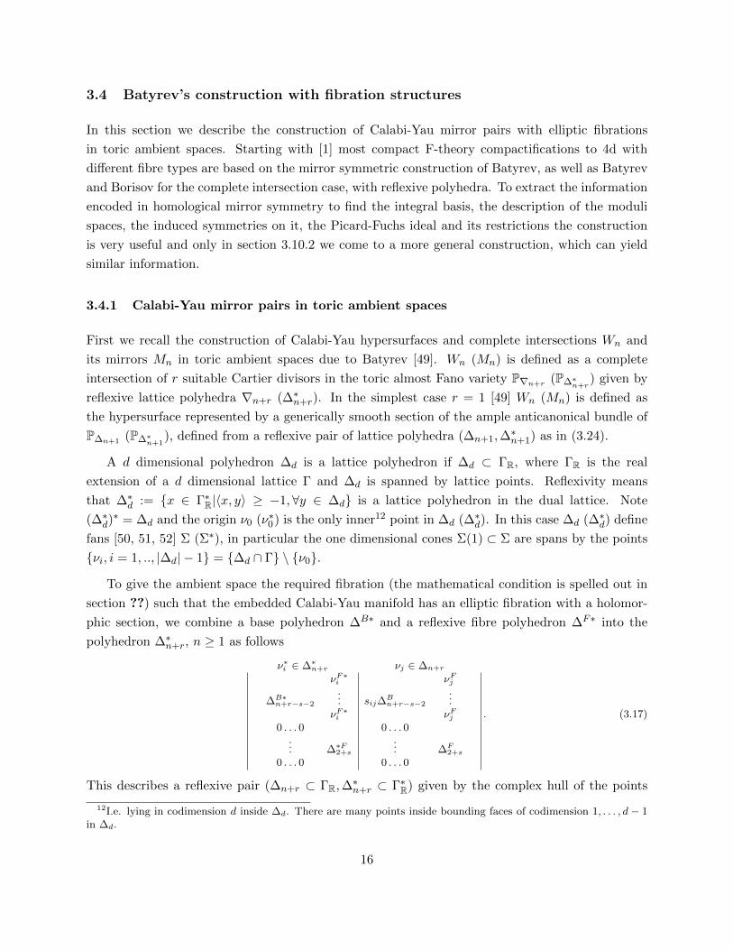
To give the ambient space the required fibration (the mathematical condition is spelled out in
section ??) such that the embedded Calabi-Yau manifold has an elliptic fibration with a holomor-
phic section, we combine a base polyhedron ∆B∗ and a reflexive fibre polyhedron ∆F∗ into the
polyhedron ∆∗n+r, n ≥ 1 as follows
ν∗i ∈ ∆∗n+r νj ∈ ∆n+r
νF∗i νFj
∆B∗n+r−s−2
... sij∆Bn+r−s−2
...νF∗i νFj
0 . . . 0 0 . . . 0... ∆∗F2+s
... ∆F2+s
0 . . . 0 0 . . . 0
. (3.17)
This describes a reflexive pair (∆n+r ⊂ ΓR,∆∗n+r ⊂ Γ∗R) given by the complex hull of the points
12I.e. lying in codimension d inside ∆d. There are many points inside bounding faces of codimension 1, . . . , d − 1in ∆d.
16
specified in (3.17). Here we defined sij = 〈νFi , νF∗j 〉 + 1 ∈ N and scaled ∆B → sij∆B. If ∆∗F
and ∆∗B are reflexive then ∆∗n+r is reflexive. For ∆∗F reflexivity is required by the desired elliptic
fibration structure. For ∆∗Bn−1 it is not a necessary condition, see [53] for more details on this
construction. In most of our general discussion of the moduli space we focus on the hypersurface
case r = 1 and s = 0 (one has always s < r), however in section 3.9.3 we find the integral
monodromy basis also for seven complete intersections and the formulas in sections 3.7, 3.10.1 and
3.10.2 apply to hypersurfaces as well as to complete intersections.
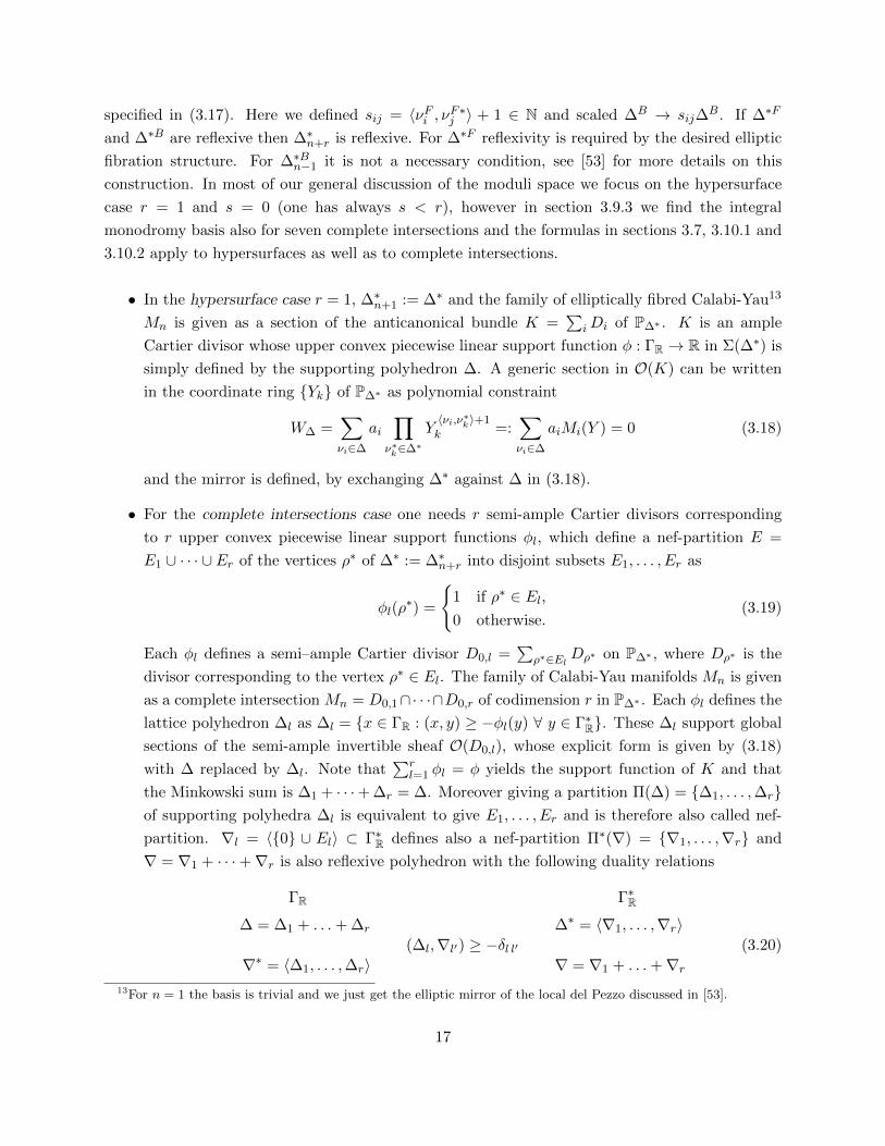
• In the hypersurface case r = 1, ∆∗n+1 := ∆∗ and the family of elliptically fibred Calabi-Yau13
Mn is given as a section of the anticanonical bundle K =∑
iDi of P∆∗ . K is an ample
Cartier divisor whose upper convex piecewise linear support function φ : ΓR → R in Σ(∆∗) is
simply defined by the supporting polyhedron ∆. A generic section in O(K) can be written
in the coordinate ring Yk of P∆∗ as polynomial constraint
W∆ =∑νi∈∆
ai∏
ν∗k∈∆∗
Y〈νi,ν∗k〉+1
k =:∑νi∈∆
aiMi(Y ) = 0 (3.18)
and the mirror is defined, by exchanging ∆∗ against ∆ in (3.18).
• For the complete intersections case one needs r semi-ample Cartier divisors corresponding
to r upper convex piecewise linear support functions φl, which define a nef-partition E =
E1 ∪ · · · ∪ Er of the vertices ρ∗ of ∆∗ := ∆∗n+r into disjoint subsets E1, . . . , Er as
φl(ρ∗) =
1 if ρ∗ ∈ El,0 otherwise.
(3.19)
Each φl defines a semi–ample Cartier divisor D0,l =∑
ρ∗∈El Dρ∗ on P∆∗ , where Dρ∗ is the
divisor corresponding to the vertex ρ∗ ∈ El. The family of Calabi-Yau manifolds Mn is given
as a complete intersection Mn = D0,1∩· · ·∩D0,r of codimension r in P∆∗ . Each φl defines the
lattice polyhedron ∆l as ∆l = x ∈ ΓR : (x, y) ≥ −φl(y) ∀ y ∈ Γ∗R. These ∆l support global
sections of the semi-ample invertible sheaf O(D0,l), whose explicit form is given by (3.18)
with ∆ replaced by ∆l. Note that∑r
l=1 φl = φ yields the support function of K and that
the Minkowski sum is ∆1 + · · ·+ ∆r = ∆. Moreover giving a partition Π(∆) = ∆1, . . . ,∆rof supporting polyhedra ∆l is equivalent to give E1, . . . , Er and is therefore also called nef-
partition. ∇l = 〈0 ∪ El〉 ⊂ Γ∗R defines also a nef-partition Π∗(∇) = ∇1, . . . ,∇r and
∇ = ∇1 + · · ·+∇r is also reflexive polyhedron with the following duality relations
ΓR Γ∗R
∆ = ∆1 + . . .+ ∆r ∆∗ = 〈∇1, . . . ,∇r〉(∆l,∇l′) ≥ −δl l′ (3.20)
∇∗ = 〈∆1, . . . ,∆r〉 ∇ = ∇1 + . . .+∇r13For n = 1 the basis is trivial and we just get the elliptic mirror of the local del Pezzo discussed in [53].
17

where the angle-brackets denote the convex hull of the inscribed polyhedra. By a conjecture
due to [54] this construction leads mirror pairs (Mn,Wn) of families of complete intersections
Calabi-Yau varieties where Mn is embedded into P∆∗ as complete intersection of the sections
W∆lof the line bundles associated to D0,l specified by ∆l, while Wn is embedded into P∇ as
complete intersection of the sections of O(D∗0,l) specified by ∇l.
For r = 0 it is explained in [49]14 how to calculate the Euler number and hn,1 and h1,1 from the
polyhedra. This determines all Hodge numbers for n ≤ 3 and for n = 4 the other Hodge numbers
follow from (3.7). The Euler number and hq,1 for 0 ≤ q ≤ d − r can also be directly calculated
by the formulas15 given for r > 0 in [54]. The above mentioned formulas relate toric divisors
and intersections thereof, as well as deformations of (3.18) to representatives in the homology
groups, while the E-polynomial [55] yields for more homology groups only information about the
dimensions.
3.4.2 Fibrations and twistings
For Calabi-Yau manifolds defined in toric ambient spaces, as above, the fibration structure descends
from a toric morphism from the ambient space. Denote by Σ the fan in Γ generated from ∆ and
by ΣB the fan defined from ∆B in the lattice ΓB (generated by ∆B) and identify PΣ with P∆ etc.
Here are the two conditions for a fibration map φ from the ambient space P∆ to P∆Bwith fibre
P∆F[50]16
• F1.) There exist a lattice morphism φ : Γ→ ΓB. This is the case if ∆F is a reflexive lattice
sub-polyhedron of the lattice polyhedron ∆ and both share the unique inner point17. The
lattice ΓF is then in the kernel of φ.
• F2.) There exists a triangulation of Σ so that every cone σ ∈ Σ is mapped under φ to a cone
σB ∈ ΣB. In this case there is an Td-equivariant morphism φ : P∆ → P∆B18.
For the manifolds described in section 3.4.1 these two criteria apply to ∆∗. It is easy to see that
the Calabi-Yau manifolds Y ⊂ P∆∗ |W∆(Y ) = 0 [56] and Y ⊂ P∆∗ |W∆1(Y ) = 0, . . . ,W∆r(Y ) =
0 [57] inherit the fibration structure from P∆∗ . In particular (3.18) is in a generalized Weierstrass
form.
A slight generalization of (3.17) is hence to chose instead of νF∗i ∈ ∆∗F with i fixed more generally
νi = (mi1, . . . ,m
i2+s) for i = 1, . . . , |∆B∗
n−1| − n. These twisting data of the fibration of P∆∗F over
14See Cor. 4.5.1, Cor 4.5.2, Thm 4.5.3.15This gives again the full Hodge diamond for n ≤ 4, which is implemented in the software package PALP.16See exercise p.49, where the statements are made at the level of the fans.17This applies in (3.17) to the quantities with and without a star.18This applies to (3.17) for the quantities with the star. It can also apply to ∆ if sij = 1.
18

P∆B∗ have a simple bound in terms of the canonical class of P∆B∗ for P∆∗ to be almost Fano [58]
or equivalently ∆∗ to be reflexive, which we discuss in section 4.1. In the heterotic/F-theory
dictionary worked out in [23] only the trivial twisting are considered and it would be interesting
to complete this dictionary. This leads in general to rational instead of holomorphic sections. I.e.
the coefficients of the fibre coordinates might be all non-trivial section over the base and one can
encounter the situation discussed above, namely that these sections all vanish at special points in
the base. In this case one gets generically non-flat fibres [59].
It is mathematically and physically useful to distinguish between flat and and non-flat fibrations.
The fibre in a flat fibration has fixed dimension, which it keeps in particular at higher codimension
loci in the base where the fibre degenerates into several irreducible components. E.g. the generic
elliptic fibre E degenerates in a flat fibration to the singular one dimensional configuration Egdescribed in section 2. In a non-flat fibration some of these components of the singular fibres
will have higher dimensions. This change of dimension can even happen for the P∆Ffibration
of the ambient space. The corresponding flatness criterium is spelled out in [60]. Let us call it
Fl1.). The question of flatness or non-flatness of the elliptic fibre is analyzed using W∆ or W∆l,
l = 1, . . . , r in the case of the complete intersections. These equations involve the coordinates of
the fibres x, y, z, w, . . ., as in (4.11,4.12,5.23,5.27) corresponding to points of ∆∗F . The monomials
M(x, y, z, w, . . .) in these coordinates are multiplied by coefficients that take value in line bundles
LM over the base and will in addition depend on ‘blow up coordinates’ corresponding to the blow
up divisors, see e.g. (5.23,5.27) 19. Let us assume that Fl1.) holds. The condition for the flatness
of the elliptic fibre Fl2.) is as follows: If these coefficients do not vanish in a sublocus of the base
so that the constraint on the fibre coordinates becomes trivial, the fibration is flat.
The toric blow up description involves adding points to ∆∗ to make it into∆∗, which adds the
corresponding ‘blow up coordinates’, see section 3.6.2. In the general terminology of resolutions
the W ∆
or W ∆l
, l = 1, . . . , r in the blow up coordinate ring are called the proper transforms of the
W∆ or W∆ldefined in the original coordinate ring.
The fibrations described by (3.17) fulfill Fl1.) and the elliptic fibrations over the almost Fano
basis described in section 4.1 and 4.2 are generically flat. However if we degenerate the complex
structure to obtain gauge groups and higher codimension structure and resolve, the elliptic fibration
might not stay flat. Examples for the flatness condition in non-toric resolution of the E8 codimension
3 singularity are discussed in section 8. Non-flat fibres are rather ubiquitous in elliptic fourfolds
with gauge groups [61].
The physical significance of the non-flat fibration is that in the limit of vanishing fibre volume
a holomorphic surface S collapses and the BPS states coming from p-branes of wrapping S as
well the holomorphic curves C inside S lead in general to a non-local quantum theory including
19In fact for the non-trivial twistings described below all monomials in the fibre coordinates might be multipliedby coefficients transforming in non-trivial line bundles over the base.
19
tensionless extended objects [62] as some light states can have electric while others have magnetic
charges as in the QFT [63]. Part of the spectrum of the tensionless string can be analyzed using
their WS CFT [64] or upon further dimensional reduction to a quantum field theory [65]. Since the
fibre is involved in the present case this is to be analyzed first in the M-theory picture, where one
gets as in [64] a (0,4)- in 5d or (0,2)-supersymmetric tensionless string in 3d from the M5 brane
wrapping S as well as an infinite tower of massless particles from M2 branes wrapping all C’s. The
infinite tower of massless states survives the M-theory/F-theory lift to 4d and can pose a thread to
F-theory phenomenology. It is not very well understood whether background fluxes can be used to
avoid the vanishing of the sections in LM or to lift the masses of these states.
3.5 The complex moduli space of toric hypersurfaces
Having immediately the mirror construction and therefore the description of the Kahler- and com-
plex moduli on the same footing is very useful to study the corresponding moduli spaces
Mcs(Mn) =MKahler structure(Wn) , (3.21)
which ultimately in the physics context one wants to lift by a superpotential. Let us focus on the
hypersurface case r = 1 and s = 0 and recall the features of W∆, the Newton polynomial of ∆d=n+1,
and its complex deformations parametrized by the ai. Its independent deformationsMW∆⊂Mcs,
whose infinitesimal directions correspond to H1(Mn, TMn), are given by a projectivization of the
ai modulo automorphisms of P∆∗20.
We want to determine possible group actions on Mcs(Mn) in order to argue that gauge sym-
metry enhancements can be induced by turning on fluxes on the invariant- or sometimes the non-
invariant periods of Mn respectively, as discussed in section 3.11. In the construction of mirror pairs
of Calabi-Yau manifolds by reflexive polyhedra and by orbifolds such group actions appear naturally
and one can define a variation of the mixed Hodge structure in terms of invariant periods on the
invariant locus S ⊂Mcs(Mn). The monodromy group acting on the periods of a family of Calabi-
Yau manifolds Mn forms a subgroup ΓM of linear integer transformations respecting a quadratic
intersection form Q on Hn(Mn,Z). For n odd the Q is symplectic and ΓM ⊂ Sp(bn(Mn),Z), which
is not necessarily of finite index for n ≥ 3, see e.g. [66] for recent progress on this question for
one parameter CY 3-folds. For n even Q is symmetric with signature σ =∫M2m
Lm (cf. (3.9)).
The realization of a group action onMcs(Mn) leads to a sub-monodromy problem on the invariant
sub-locus S ∈ Mcs for which ΓS ⊂ ΓM can e.g. be a finite index subgroup in products of SL(2,Z)
as in the example in section (5.2.1). Studying the various ΓSi is obviously an important tool to
20These are called monomial deformations in the complex moduli space or toric deformations in Kahler mod-uli space. There can be non-monomial (non-toric) deformations which indicated in brackets whenever we specifyh1(Mn, TMn) ∼ hn−1,1(Mn) = #monomial(#non − monomial) or h1,1 = #toric(#non − toric). Note that themonomial deformations define a good subspace inMcs(Mn) and in the following we assume for simplicity that thereare no non-monomial deformations.
20

get a handle on ΓM, with many implications, e.g. that the functions that determine the effective
action in section 3.8 are organized in terms of automorphic forms w.r.t. ΓSi . In all known cases
the variation of the mixed Hodge structure related to ΓS is the variation of mixed Hodge structure
of an actual geometry. Either of a Calabi-Yau manifold Mn of the same dimension possibly after
a transition or, if the flux violates the tadpole condition (3.15) and decompactifies Mn, of a lower
dimensional geometry, e.g. a Seiberg-Witten curve or a lower dimensional Calabi-Yau manifold. It
is clear that the tadpole condition (3.15) cannot be realized in general on both sides of a transition
without tuning the fluxes. The simplest examples are transitions between Calabi-Yau manifolds
where χ mod 24 differs on both sides. From the pure geometrical point of view such transitions
are possible [1]. A detailed analysis of this question of fluxes in local transitions has been made
in [30]. In the applications in F-theory moduli stabilization it however is not necessary to actually
go through the transition. We just want the moduli to settle close to the transition point.
To describeMcs it is useful to extend the spaces in which the polyhedra live by one dimension
and to define (∆, ∆∗) as the embedding of (∆,∆∗) in hyperplanes H at distance one from the origin,
i.e. as the complex hull of νi := (νi, 1) and ν∗i := (ν∗i , 1). Each of the k = |∆∗| − (d + 1)
linear relations ∑i
ν∗i l∗(p)i = 0, p = 1, . . . , k , (3.22)
with l∗(p)i ∈ Z and
∑i l∗(p)i = 0 between the points of the polyhedron ∆∗ yields an action of C∗ on
the coordinates of Yj defined by
Yj 7→ Yjµl∗(p)jp , j = 1, . . . , |∆∗| − 1 , (3.23)
with µp ∈ C∗ under which W∆ = 0 has to be invariant21. The latter property defines it and is
necessary make it well defined in the ambient space
P∆∗ = (C[Y1, . . . , Yk=|∆∗d|−1] \ SR∗)/G, (3.24)
where G = HomZ(Ad−1,C∗). The Chow group Ak is generated by the orbit closures of d − k
dimensional cones. I.e. Ad−1 is generated by one dimensional cones Σ(1), which are the Weyl
divisor modulo linear equivalence. Hence for reflexive polyhedra G = (C∗)|∆∗|−(d+1) ×Gtor, where
the finite group Gtor = HomZ(An−1(P∆∗)tor,Q/Z) and (C∗)|∆∗|−(d+1) is generated by (3.23). The
Stanley-Reisner ideal SR∗ depends on a subdivision S∗ of Σ∗ into d-dimensional simplicial cones
Σ(d) of volume 1 in Γ∗, the toric description of resolving the singularities of P∆∗ completely22.
From this subdivision the Stanley Reisner ideal is given simply combinatorial: Let I∗ be any index
21If one keeps Y0 where ν∗0 = 0 is the origin then W∆ itself is invariant, not just its vanishing locus.22A coarse subdivision S∗c is given by a complete subdivision of ∆∗ into d-dimensional simplices, where each simplex
has the origin as a vertex. Not all simplicial cones obtained in this fashion have volume 1, so that rays through pointsoutside ∆∗ have to be added to make P∆∗ smooth, however W∆ = 0 misses the corresponding singularities and isalready smooth with the coarse subdivision.
21
set of points in ∆∗ with |I∗| ≤ d then the Bd−|I∗| = Di1 ∩ . . .∩Di∗|I|= (Yi∗1 = 0∩ . . .∩Yi∗|I∗| = 0
is in SR∗, iff ν∗i1 , . . . , ν∗i|I| are not in a cone Σ(|I∗|) of S∗.
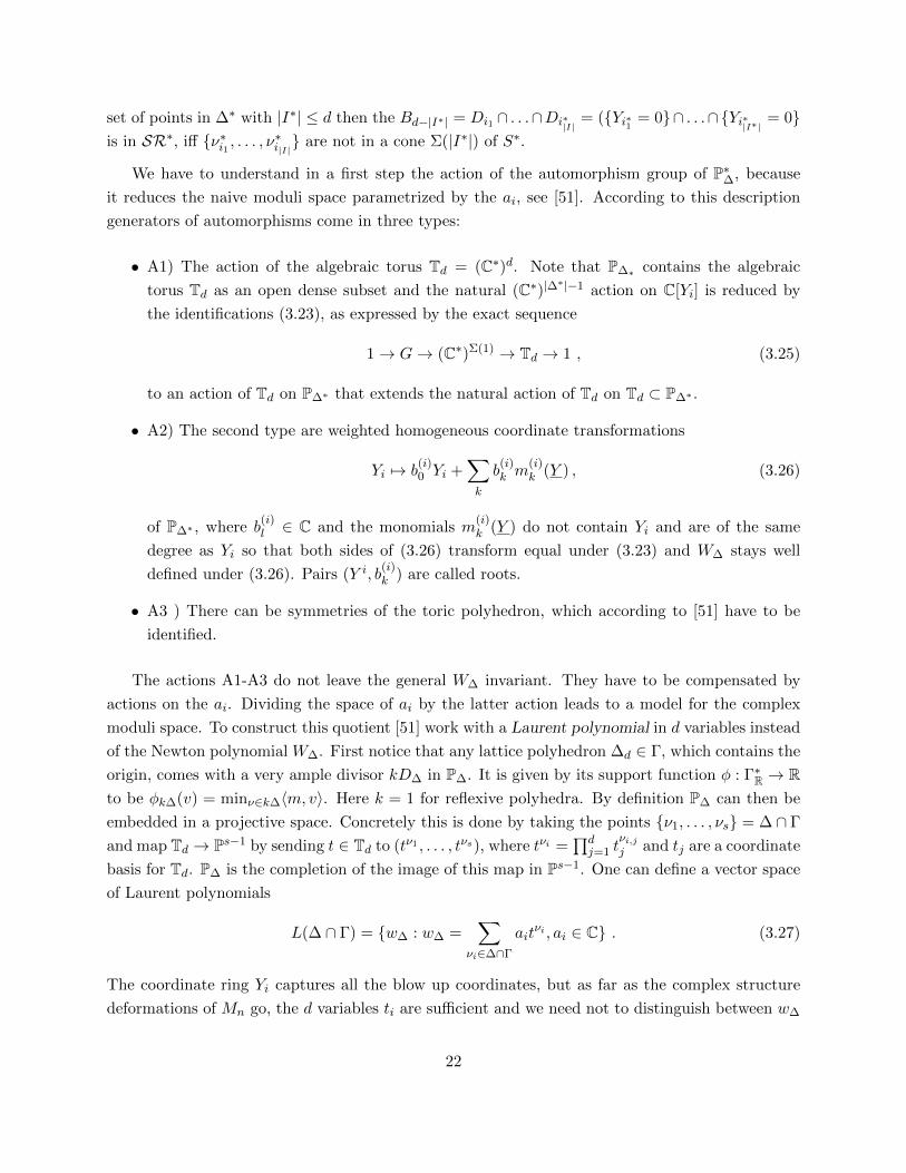
We have to understand in a first step the action of the automorphism group of P∗∆, because
it reduces the naive moduli space parametrized by the ai, see [51]. According to this description
generators of automorphisms come in three types:
• A1) The action of the algebraic torus Td = (C∗)d. Note that P∆∗ contains the algebraic
torus Td as an open dense subset and the natural (C∗)|∆∗|−1 action on C[Yi] is reduced by
the identifications (3.23), as expressed by the exact sequence
1→ G→ (C∗)Σ(1) → Td → 1 , (3.25)
to an action of Td on P∆∗ that extends the natural action of Td on Td ⊂ P∆∗ .
• A2) The second type are weighted homogeneous coordinate transformations
Yi 7→ b(i)0 Yi +
∑k
b(i)k m
(i)k (Y ) , (3.26)
of P∆∗ , where b(i)l ∈ C and the monomials m
(i)k (Y ) do not contain Yi and are of the same
degree as Yi so that both sides of (3.26) transform equal under (3.23) and W∆ stays well
defined under (3.26). Pairs (Y i, b(i)k ) are called roots.
• A3 ) There can be symmetries of the toric polyhedron, which according to [51] have to be
identified.
The actions A1-A3 do not leave the general W∆ invariant. They have to be compensated by
actions on the ai. Dividing the space of ai by the latter action leads to a model for the complex
moduli space. To construct this quotient [51] work with a Laurent polynomial in d variables instead
of the Newton polynomial W∆. First notice that any lattice polyhedron ∆d ∈ Γ, which contains the
origin, comes with a very ample divisor kD∆ in P∆. It is given by its support function φ : Γ∗R → Rto be φk∆(v) = minν∈k∆〈m, v〉. Here k = 1 for reflexive polyhedra. By definition P∆ can then be
embedded in a projective space. Concretely this is done by taking the points ν1, . . . , νs = ∆ ∩ Γ
and map Td → Ps−1 by sending t ∈ Td to (tν1 , . . . , tνs), where tνi =∏dj=1 t
νi,jj and tj are a coordinate
basis for Td. P∆ is the completion of the image of this map in Ps−1. One can define a vector space
of Laurent polynomials
L(∆ ∩ Γ) = w∆ : w∆ =∑
νi∈∆∩Γ
aitνi , ai ∈ C . (3.27)
The coordinate ring Yi captures all the blow up coordinates, but as far as the complex structure
deformations of Mn go, the d variables ti are sufficient and we need not to distinguish between w∆
22

and W∆23. The statement about the moduli space can now be phrased as
MW∆= P(L(∆ ∩ Γ))/Aut(P∆∗) . (3.28)
It has been further shown by Batyrev that any complex structure deformation has a represen-
tative under the (gauge) orbits (3.26), which corresponds to the restricted Newton polynomial of ∆
in which only such monomials in (3.18) are considered that correspond to points in ν(i) not inside
co-dimension one faces of ∆, we call ∆ without those points ∆0. This can be viewed as a gauge
fixing. This leads to the definition
MsimpW∆
= P(L(∆0 ∩ Γ))/Td, (3.29)
and one can show that the map φ : MsimpW∆
→ MW∆is at most a finite cover. Note that not all
symmetries of Mn might be manifest in a chosen gauge.
As it turns out the most interesting points in the analysis below are precisely related to the
nature of the finite covers. In order to get the right description for Mcs we propose to divide
Aut(P∆∗) by the discrete group G described in section 3.6.
3.5.1 Large complex structure coordinates and the point of maximal unipotent mon-odromy
One can introduce coordinates, which eliminate the Td=n+1 × C∗ action (the C∗ action is the one
that scales W∆)
zk = (−1)l(k)0
|∆0|∏i=0
al(k)ii , ∀k = 1, . . . , |∆0| − (d+ 1) = hn−1,1 . (3.30)
A mirror conjecture of Batyrev states that if the l(k) are the vectors spanning the Mori cone of P∆,
which descends to Wn, then zk = 0 ∀k is a point of maximal unipotent monodromy in the complex
moduli space of Mn, which maps under the mirror map to a large volume point of Wn inside the
Kahler cone of P∆. The topological data of Wn determine the degenerations of the period vector at
this point, which is not the the only but the most important datum to fix an integral basis for the
periods. The Kahler cone is dual to the Mori cone. In the case of toric varieties P∆, the Mori cone
can be calculated from a maximal star (Kahler) triangulation of ∆ 24 and of course due to mirror
symmetry the formalism described in great detail in [52] for the Kahler cone applies on both sides.
23Physically this independence of complex parameters from the blow ups moduli reflects, e.g. the decoupling ofvector- and hypermultiplets in type IIb compactifications on M3 to 4d at generic loci in the moduli space.
24As encoded in the secondary fan, there can be many Kahler triangulations of ∆ and correspondingly many pointsof maximal unipotent monodromy in the family Mn.
23

3.6 Group action on Mcs(Mn)
Now that we have a model forMcs(Mn) we can come to the main point namely the induced group
actions on it.
3.6.1 Discrete group actions and Orbifolds
Group actions onMcs can be induced from symmetry acting on Mn. Generic Calabi-Yau manifolds
with full SU(n)-holonomy have no continuous symmetries, but one easily finds discrete symmetry
groups G acting on them. To define a Calabi-Yau orbifold, whose moduli space is the invariant
subspace S ⊂ Mcs, they have to leave the holomorphic (n, 0)-form Ωn invariant. The latter con-
dition implies that G acts like a discrete subgroup of SU(n) in each coordinate patch of Mn. For
n < 4 this guarantees that the fixed sets of the G action on Mn can be geometrically resolved
without changing the triviality of the canonical class, i.e. maintaining the CY condition on the
resolved space Mn/G . For n = 4 there can be terminal singularities remaining on the CY orb-
ifold, which do not render string and F-theory compactifications inconsistent. Dividing discrete
symmetries and resolving the singular space if the symmetries have fix sets to Mn/G was described
in [67] in comparison with symmetries that lead orbifolds of Gepner models with (2, 2) world-sheet
supersymmetry. For the latter the condition G ⊂ SU(n) ensures that the (2, 2) super charges are
not projected out. The symmetries considered in [67] act on the ambient space coordinates with
two properties
• G1.) They leave W∆ invariant in the sense that they can be compensated by an action on
the ai1
• G2.) They leave µ defined in (3.48) invariant1.
The geometrical condition G2.) is controlled by the explicit form (3.48) for toric varieties with a
dominant weight vector 25. For example, G can be generated by phases αnk = exp(2πin/k), k, n ∈ Zacting on the coordinates as xi 7→ αnik xi, i = 1, . . . , n+2 where
∏i α
nik = 1 or by even permutations
on coordinates with equal weights. Such permutation orbifolds including non-abelian orbifolds have
been considered in [68]. These permutations are special cases of discrete root operations (3.26),
which can contain more general generators. It was observed in [69] that dividing the maximal
phase symmetry group Gmaxph from Fermat hypersurfaces yields a mirror geometry26 M3/Gmaxph , a
statement that can be generalized to higher dimensional Mn.
1Up to scaling λ ∈ C∗.25In the general case one can control this condition by establishing an Etale map between two reflexive toric
polyhedra.26This a special case of Batyrev’s construction and an example is discussed in section 3.11.1.
24

The G action G : Mn → Mn induces an action G∗ : H∗(Mn) → H∗(Mn) and properties of this
map are captured by the Lefschetz fixed-point formulas. Here we need a much more trivial fact.
The above G∗ action will decompose Hn(M,Z) in cyclic orbits of finite length. Let us focus on one
divisor of |G| and denote the orbit of length k by
Γ0 7→ Γ1 7→ . . . 7→ Γk−1 7→ Γ0 . (3.31)
Note that there can be relations in homology among the cycles Γi. The eigenvectors with eigenvalue
(αk)p in this orbit are Γdiagp = 1
k
∑k−1l=0 (αk)
l(k−p)Γl with αk the elementary k’th root of unity. I.e.
Γdiag0 , the invariant cycle can be defined after rescaling in Hn(M,Z), but to diagonalize the non-
invariant cycles Hn(M) w.r.t. to G if k is prime and there are no homological relations, one has to
extend the number field Z to Z⊕ αk27.
We assume now that the automorphisms Tn+1 × C∗ and A2.) have been fixed to leave ai,
i = 1, . . . , hn−1,1 as coordinates on M simpW∆
. G1.) defines an action G : MsimpW∆
→ MsimpW∆
. Let
us consider a generator of order k, i.e. a phase action g : xi 7→ αnik xi that rotates monomials
Mi → αmik Mi in W∆ by a nontrivial k-th root of unity. For simplicity we first assume k to be
prime. Latter on we discuss implications if that is not the case. The phase rotations induce an
action on the non-invariant moduli ai
g : ai → α−mik ai . (3.32)
Let us call W inv∆ =
∑k
aiM
invk the polynomial containing only invariant monomials. We assume
that W inv∆ = 0 is transversal, i.e. dW inv
∆ = 0 and W inv∆ = 0 have generically no solution, to have
a good sub-monodromy problem. By Bertinis-theorem this can be checked on the base locus of
P∆∗ . A combinatorial criterium is given in [70] and is equivalent to the condition that W inv∆ is the
Newton polynom of a reflexive polyhedron.
Now note that the action of g (3.32) is not visible in the coordinates (3.30). This is due to
the fact that the actual moduli space is parametrized by the ai variables that multicover the zi.
Let Πp =∫
ΓpΩ, p = 0, . . . , k − 1 be periods over the cycles Γp, p = 0, . . . , k − 1 in (3.31). We
like to study them as solutions of the Picard-Fuchs differential system and their dependence on
one non-invariant modulus a on which g acts by (3.32) near the orbifold point in the moduli space
a = 0. Here their power series expansion has to have the form Πp =∑∞
n=0 cn(a)(aαpk)n. The
occurrence of αk is necessary to realize the transformation (3.31). The cn(a) depends on moduli
that do not transform under the generator g and contains in particular the totally invariant moduli
under G which we calla. Since by assumption W inv
∆ = 0 is transversal c0(a) 6= 0 for generic a.
Otherwise the invariant period would vanish generically on S, in contradiction to the assumption.
27 In fact extending the number field is an interesting logical possibility. It would still represent a discrete choiceof fluxes and if the flux disappears at the attractor point there seems no physical contradiction.
25

One concludes that the series expansion of the periods Πdiagp near a = 0 is
Πdiagp =
∞∑n=0
cp+kn(a)ap+kn, p = 0, . . . , k − 1 . (3.33)
Let zi be a variable in the base, which is by (3.30) k-times covered by the ai on which (3.32) act.
Then the periods Πp over the non-invariant cycles Γp, p = 1, . . . , k−1, will have the typical orbifold
behaviour at S, i.e. they go in leading order with Πdiagp = z
p/ki +O(z
p/k+1i ), p = 0, . . . , k − 1. We
can conclude some more facts. The monodromy MZk ∈ ΓM around S is of order k and acts on k−1
integer periods, which span a subspace of all periods. The invariant submoduli space S ⊂MW∆is
the vector space L(∆inv ∩ Γ) divided by G invariants roots (xi, b(i)k ) and Tn+1 × C∗/G.
We have further seen that the relevant automorphism group is
Aut(W∆) = Aut(P∆∗)/G , (3.34)
where G is the maximal group obeying G1) and G2). Accordingly we define the moduli space of
the polynomial deformations as
MW∆= P(L(∆ ∩ Γ))/Aut(W∆) . (3.35)
This has the correct multicovering structure and we get an induced group action of G on MW∆as
well as on the periods
Π(ga) = MgΠ(a) . (3.36)
In particular Mg acts on Γ in Hn(Mn) as a monodromy matrix respecting the dual intersecting
pairing
Q∗(MgΓ,MgΓ) = Q∗(Γ,Γ) . (3.37)
E.g. if n is odd Mg is a symplectic matrix in SP(bn,Z). We assumed in (3.33) that there are no
homological relations between the Γp. In compact cases there will be generically such relations
and one has to calculate the transition matrix between the local basis Γp, p = 0, . . . , k − 1 and the
global integral basis, see e.g. (3.113). Since G is globally defined one expects this matrix to be
rational rather than transcendental. This is one key ingredient to have an integral superpotential
that drives the moduli to the orbifold point and will be established rigorously for important general
cases in section 3.10.2. For the sextic and other one parameter models we establish this fact as
well as (3.37) explicitly for fourfold orbifolds e.g. in (3.105). Many threefold cases can be found
in [71, 72]. E.q. (3.37) means that the Kahler potential (3.57) is monodromy invariant.
The ideas discussed in this section are related to a general principle to characterize the mon-
odromy group ΓM(Mn) of a family of Calabi-Yau manifolds Mn by the monodromy group ΓM(Un) of
a more universal family of Calabi-Yau manifolds Un, whose generic member has a smaller symmetry
group G(Un) ⊂ G(Mn), as
ΓM(Mn) ∼ ΓM(Un)G(Un)
G(Mn). (3.38)
26
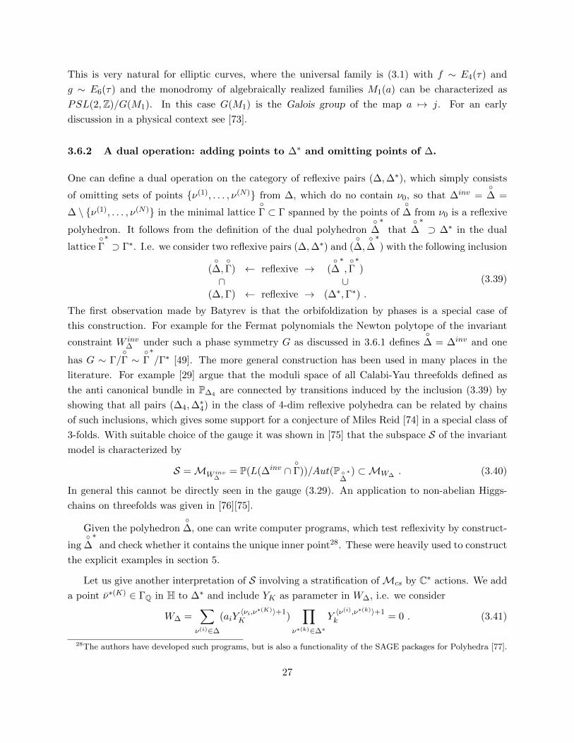
This is very natural for elliptic curves, where the universal family is (3.1) with f ∼ E4(τ) and
g ∼ E6(τ) and the monodromy of algebraically realized families M1(a) can be characterized as
PSL(2,Z)/G(M1). In this case G(M1) is the Galois group of the map a 7→ j. For an early
discussion in a physical context see [73].
3.6.2 A dual operation: adding points to ∆∗ and omitting points of ∆.
One can define a dual operation on the category of reflexive pairs (∆,∆∗), which simply consists
of omitting sets of points ν(1), . . . , ν(N) from ∆, which do no contain ν0, so that ∆inv =∆ =
∆ \ ν(1), . . . , ν(N) in the minimal latticeΓ ⊂ Γ spanned by the points of
∆ from ν0 is a reflexive
polyhedron. It follows from the definition of the dual polyhedron∆∗
that∆∗⊃ ∆∗ in the dual
latticeΓ∗⊃ Γ∗. I.e. we consider two reflexive pairs (∆,∆∗) and (
∆,∆∗) with the following inclusion
(∆,Γ) ← reflexive → (
∆∗,Γ∗)
∩ ∪(∆,Γ) ← reflexive → (∆∗,Γ∗) .
(3.39)
The first observation made by Batyrev is that the orbifoldization by phases is a special case of
this construction. For example for the Fermat polynomials the Newton polytope of the invariant
constraint W inv∆ under such a phase symmetry G as discussed in 3.6.1 defines
∆ = ∆inv and one
has G ∼ Γ/Γ ∼
Γ∗/Γ∗ [49]. The more general construction has been used in many places in the
literature. For example [29] argue that the moduli space of all Calabi-Yau threefolds defined as
the anti canonical bundle in P∆4 are connected by transitions induced by the inclusion (3.39) by
showing that all pairs (∆4,∆∗4) in the class of 4-dim reflexive polyhedra can be related by chains
of such inclusions, which gives some support for a conjecture of Miles Reid [74] in a special class of
3-folds. With suitable choice of the gauge it was shown in [75] that the subspace S of the invariant
model is characterized by
S =MW inv∆
= P(L(∆inv ∩Γ))/Aut(P
∆∗) ⊂MW∆
. (3.40)
In general this cannot be directly seen in the gauge (3.29). An application to non-abelian Higgs-
chains on threefolds was given in [76][75].
Given the polyhedron∆, one can write computer programs, which test reflexivity by construct-
ing∆∗
and check whether it contains the unique inner point28. These were heavily used to construct
the explicit examples in section 5.
Let us give another interpretation of S involving a stratification ofMcs by C∗ actions. We add
a point ν∗(K) ∈ ΓQ in H to ∆∗ and include YK as parameter in W∆, i.e. we consider
W∆ =∑ν(i)∈∆
(aiY〈νi,ν∗(K)〉+1K )
∏ν∗(k)∈∆∗
Y〈ν(i),ν∗(k)〉+1k = 0 . (3.41)
28The authors have developed such programs, but is also a functionality of the SAGE packages for Polyhedra [77].
27

The point ν∗(K) ∈ H defines a new linear relationl(r+1)
in 〈∆∗, ν∗(K)〉, which we let act in the
usual fashion on all Yi by (3.23). Under this scaling µk the constrained W∆ is not invariant.
It can be kept invariant by rescaling the ai. This defines uniquely an C∗-action on the moduli
spaceµK : MW∆
→ MW∆. Moreover the fixed locus of the induced action on MW∆
is simply
defined by setting the coefficients ai of those monomials to zero, which are not invariant under
µk. In general we add several points ν∗(K), K = 1, . . . , N∗ and get N∗-actionsµK , whose fixed
locus is is obtained by setting more coefficients ai to zero. The invariant polynomial is W∆inv and∆∗
= 〈∆∗, ν∗(1), . . . ν∗(N)〉 is a new lattice polyhedron in the new latticeΓ∗. The characterization
of the fix point locus S is again given by (3.40).
We claim that S is a good subspace of S ⊂ MW∆in the following sense. The Gauss Manin
connection closes on S for a subset of invariant periods. The monodromy group acting on the
invariant periods Γ is a proper subgroup of ΓMcs . This will be further discussed in section (3.7).
Of course by mirror symmetry there is a dual inclusion of the quantum corrected Kahler moduli
space S∗ = MW∆∗ = P(L(∆∗ ∩Γ∗))/Aut(P∆) ⊂ MW ∗
∆
. For future reference we will call the
manifold defined as anticanonical bundle in P ∆
asMn.
3.7 The variation of Hodge structures: degenerations and sub-monodromy sys-tems
The primitive horizontal subspace in the cohomology of a Calabi-Yau n-fold Mn comes with a
polarized Hodge structure, see [51][78][79] for reviews. For families of Calabi-Yau n-folds π :
Mn → Mcs over their complex moduli space Mcs with fibre π−1(t) = Mt one captures the
Hodge decomposition Hn(M,C) = ⊕nk=0Hn−k,k with Hp,q(M) = Hq,p(M), with respect to the real
structure Hn(Mn,R), in terms of Hodge filtrations29 F • = F pnp=0 with F p = ⊕pl≥pHl,n−l so that
F p ⊕ Fn−p+1 = Hn(M,C) , Hp,q(M) = F p(M) ∩ F q(M) and Hp,q(M) = F p/F p+1. Together
with the lattice Hn(Mn,Z) this defines the Hodge structure. Unlike the Hp,q(Mn) the Fp(Mn)
vary holomorphically with the complex structure and fit into locally free sheaves with inclusion
Fp ⊂ Fp−1, which defines a decreasing or Hodge filtration. In particular F0 = Rnπ∗C ⊗ OMcs is
the Hodge bundle H, which has a locally constant subsheaf Rnπ∗C. Taking this as the flat section
of F0 defines a flat connection, called the Gauss Manin connection
∇(s⊗ f) = s⊗ df . (3.42)
The Gauss Manin connection fulfills the Griffiths transversality
∇Fp ⊂ Fp−1 (3.43)
29Sometimes, especially in the physics literature, Fp = Fn−p is used.
28

and is equivalent to the Picard-Fuchs differential ideal IPF , which is the kernel of the map
φ(X1, . . . , Xr) = ∇X1 . . .∇XrΩ(t) from the sheaves of linear differential operators Di on Mcs to the
Hodgebundle F0, which makes the latter into a D-module. Here Xi = ∂ai , i = 1, . . . , r = dim(Mcs)
is a basis of vector fields on Mcs. As
∂ai
∫Γt
Ω(t) =
∫Γt
∇∂aiΩ(t) (3.44)
the Di annihilate the periods and determine them.
D-modules are a notion to study monodromy systems. In particular they were used in [80, 81]
to prove the Riemann-Hilbert problem for holonomic system in more variables, see [82] for a review.
A criterium when the Di generate IPF was given in [83]: This is the case if the symbols of the
ideal IPF at a point of maximal unipotent monodromy of Mn determine the classical intersection
ring of Wn up to one normalization, see (3.143). Iff this is the case, then one can obtain exactly
all 3-point couplings from IPF using Griffiths transversality [83]. These exact couplings are in the
A-model language the fully instanton corrected ones. A sub-monodromy system is in this language
a restriction of the dependent variables onto a subspace S ⊂ Mcs, so that IPF |S is Picard-Fuchs
ideal of another Calabi-Yau geometry. This restricts the D-modul to sub-modul and the restricted
Calabi-Yau geometry stays compact, if the period of the Hodge bundle that maps to the structure
sheaf of Wn restricts to a period contained in the sub-modul, otherwise the restricted Calabi-Yau
geometry becomes non-compact.
The hn(Mn) solutions of the Picard-Fuchs equations are independent sections of the Hodge
bundle that extend globally over all Mcs. We group the solutions into the period vector Π(a) =
(∫
Γ1Ωn(a), . . . ,
∫Γbn
Ωn(a))T . Because of the flatness of ∇ the relevant data determining Π(a)
and (also the dual Π(a), see (3.56)) are the monodromies of Π(a) around the components of the
discriminant locus ∆ = 0 in Mcs. The latter has to be resolved to Mcs so that the components
∆i = 0 of ∆ = 0 have all normal crossings and the monodromies can be defined. The theorem
of Landman describes the behavior of the periods at ∆ = 0. Essentially they can have at most
log(∆i)n singularities and/or finite order k branch cuts. This is encoded in (Lefschetz) monodromy
matrix Mi that describes the transport of Π(a) around ∆i = 0. Landman’s monodromy theorem
states that Mi has the property [84]
(Mki − 1)p+1 = 0, with p ≤ n . (3.45)
Here p is the smallest integer so that the r.h.s. is zero. For p = 0, k > 1 one has an Zk orbifold
singularity. The case is discussed in sections 3.6.1 and 3.11.1. The cases k = 1 are the unipotent
cases. The conifold in n odd has p = 1 and the most relevant case for mirror symmetry is the
maximal unipotent case p = n. Mixed cases are also relevant in physics, e.g. the SU(N) Seiberg-
Witten embedding has in the asymptotic free region k = N and n = 1. The degeneration of the
Hodge structure is studied extensively in mathematics. However this is still a local analysis and
29

as such a linear analysis. In order to enjoy the full modularity properties of the amplitudes like
the superpotential one has to do the global construction outlined in section 3.9.2 and 3.9.3. An
intermediate concept is local mirror symmetry, which deals with a sub-monodromy problem of the
finite periods in a semi local limit, where part of Mn decompactifies, see (3.144) and section (5.2.1).
As a local analysis we recall as a simple example the limiting mixed Hodge structure for the
unipotent cases, see [85][78] for review. Let zi ∼ ∆i be the coordinates on the ith punctured disk
Di so that (D)r is a local neighborhood at a normal crossing point. The mixed case is reduced
to unipotent case by changing to multicover variabels z1k 7→ z. Since Ni = Mi − 1 is nilpotent one
can define the Lie algebra generator Ni = log(Mi) as a finite expansion in Ni. Ni and Ni have the
same kernel and cokernel. Schmid’s nilpotent orbit theorem [86] provides an extension Fp of Fp
from (D)r to the product of full disks Dr. In particular he extends the Gauss Manin connection to
a map ∇ : F0 → F0⊗Ω1Mcs
(log(∆i)). Here the sheaf of rational one forms Ω1Mcs
(log(∆i)) is in the
case of l unipotent divisors locally generated by dz1z1, . . . , dzl
zl, dzl+1, . . . ,dzr. On Dr he introduces
single valued periods
ΠS(z) = exp
(− 1
2πilog(zi)Ni
)Π(0) , (3.46)
extends that to a section of Fp and shows that this is a leading order approximation to the periods
on the disk. From the degenerations of the periods found in mirror symmetry calculations that
is no surprise and contrary to the claim in [87] it gives not a very useful approximation to the
superpotential as it misses the terms from the Γ class in the periods, i.e. not only terms that are
exponentially suppressed, but for the fourfolds terms that actually diverge logarithmically at z = 0.
An important implication of the work of [86][88] is the ability to define the limiting mixed
Hodge structure, which describes how the integral Hodge structure of the singular model sits inside
the integral Hodge structure of the smooth case. In particular at 0 ∈ Dr there is a limiting
Hodge filtration F• = F•lim with Nj(Fplim) ⊂ Fp−1lim . Both Ni and the extension ∇θzj (F
plim) ⊂ Fp−1
lim
induce a linear map Fplim/Fp−1lim 7→ Fp−1
lim /Fplim and are identified as ∇θzj = − 12πiNj . Moreover if
ΠS(z) is a multivalued flat integer section of HZ then ΠS(0) is an integral element over 0. The
mixed Hodge structure comes from the monodromy weight filtration W • with W0 ⊂ W1 ⊂ . . . ⊂W2n = Hn(Mt,C). For any linear combination N of the Ni with strictly positive coefficients
one defines W0 = Im(N),W1 = Im(Nn−1) ∩ Ker(N),W2 = Im(Nn−2) ∩ Ker(N) + Im(Nn−1) ∩Ker(N2), . . . ,W2n−1 = Ker(Nn). Let Grk = Wk/Wk−1. It is easy to see that N(Wk) ∈Wk−2 and it
follows from the Jacobson-Morozov Lemma that Nl : Grk+l ∼ Grk−l. Much more non-trivially F•limis a Hodge structure of weight k on Grk, which means that (F•lim,W•) is a mixed Hodge structure.
It can be shown that N is the lowering operator of a SL(2,C) action on the LMHS [86].
The easiest example is the nodal degeneration of a genus g Riemann surface Σg. One can chose
a symplectic basis Ai, Bi i = 0, . . . , g − 1 such that A0 degenerates. By the Lefschetz formula
(3.166 the only cycle which is not monodromy invariant is M : B0 7→ A0 +B0. N = N is nilpotent
N2 = 0. One has N : B0 7→ A0 while all others cycles are annihilated. W−1 := 0, so Gr0 = Q · A0
30

of grade 0 must be of type (0, 0), Gr1 = spanQA1, . . . , Ag−1, B1, . . . , Bg−1 = Hn(Σg−1,Q) and
Gr2 = Q · B0 of grade 2 must be of type (1, 1). I.e. over Q the cohomology of Σg splits and on
Hn(Σg−1,Q) and one has a closed sub-monodromy problem on the latter. The situation is very
similar for the conifold transition in Calabi-Yau 3-folds, up to the fact that in a real transition m
S3 with r relations shrink [89].
Another typical situation in which a sub-monodromy problem arises is for the central fibre in a
stable degeneration limit, see section 5.2.1 for the explicit solution of the latter for the limhetK3 =
dP9 ∪T 2 dP9 example. In addition to the limiting mixed Hodge structure described above, the
Clemens-Schmid exact sequence relates the Hodge structure on the central fibre to the one of the
smooth space, see D. Morrison’s article in [79] for a review and [89] for examples. The approach
to glue in the complex degeneration limit two or more components of Mn with positive first Chern
class along the central fibre with vanishing first chern class is a very old idea from perspective of
Gromov-Witten invariants on Mn, as the latter are deformation invariant and the calculation in
the degeneration limit is at least possible. There has been a lot of recent progress in this program
by Gross and Siebert, see [90] for review. Maulik and Pandharipnade used it to get information
about higher genus invariants on the degenerate quintic, where the central fibre is a K3. However
working purely in the A- model with relative Gromov-Witten invariants is combinatorial extremely
complicated and the authors obtain explicitly only the degree 1 genus two Gromov-Witten invariant
on the quintic [91]. It is reasonable to assume that the B-model perspective, i.e. the modularity
in the sub-mondromy problem and integrality of the BPS invariants is of great help to tackle the
combinatorics. In fact Maulik, Pandharipande and Thomas [92] use this approach in the stable
degeneration limit of F-theory to the heterotic string, discussed more in section 5.2.1, where the
modular properties are best understood, to prove integrality of the BPS invariants.
In order to use the localization argument w.r.t. to the group action G its fix points S must be
a sub locus in Mcs that leads to a well defined variation of the Hodge structures of the invariant
periods. If we include all orbifold divisors in ∆ then S ∈ ∆ then S ⊂ ∆. This structure in particular
defines a sub-monodromy problem in the invariant subspace S. We therefore discuss in the rest of
the section two and a half methods for deriving the differential ideal IPF that makes the occurrence
of the sub-monodromy problem obvious in the hypergeometric case.
• (i) Gelfand-Graev-Kapranov-Zelevinsky method: The “periods”
Πi(a) =
∫Γi
Ωn =
∫Γi
∮γ
µ
W∆(x, a), (3.47)
31

where γ is a path in P∆∗ around W∆ = 0, Γi ∈ Hn(Mn,Z) and 30
µn+1 =n+1∑j=1
(−1)jwixjdx1 ∧ . . . ∧ dxj ∧ . . . dxn+1 , (3.48)
are annihilated by a restricted set of GKZ differential operators of [93, 94] appropriate for
the resonant case
Dl(k) =∏l(k)i >0
(∂
∂ai
)l(k)i
−∏l(k)i <0
(∂
∂ai
)−l(k)i
, Zi =
r∑j=0
νj,iθj − βi , (3.49)
where 1 ≤ k ≤ |∆0|−d−1 , 1 ≤ i ≤ n+1, r = |∆0| and β = (−1, 0, . . . , 0) and θi = ai∂∂ai
. The
first set of operators k = 1, . . . , h11(W ) follows from the linear relation between the points
in ∆, which are encoded in l(i) obtained from an analogous construction to the one that
lead to (3.22). The second set of operators j = 0, . . . , d eliminates the C∗ scaling symmetry
of W∆ and the Td redundancy A1) in the parametrization of Mcs in terms of the ai. It was
observed in [83] that (3.49) are sufficient to solve model of type I and that for type II models
the infinitesimal version of the invariance of (3.47) under each transformation corresponding
to the roots (3.26) leads to first order differential operators Z ′k, which supplement (3.49)
and that for general type III models one needs further differential equations Z ′′k coming from
relations between monomials corresponding to points at height modulo ∂iW∆. Such relation
can be found algorithmically using the Groebner basis for the Jacobian ideal J , see below.
The main advantage of using the differential symmetry (3.49) is that solutions can be very
explicitly written down near the large complex structure point z = 0, where z(a) is defined
in (3.30). One finds [95] with the definition
ω0(z, ρ) =∑n
c(n, ρ)zn+ρ where c(n, ρ) =
∏j Γ(∑
α l(α)0j (nα + ρα) + 1)∏
i Γ(∑
α l(α)i (nα + ρα) + 1)
(3.50)
that ω0(z, ρ)|ρ=0 is a solution and all other solutions are given by derivatives w.r.t. ρi at ρ = 0
by the Frobenius method, see section 3.9.2. Note that in formula (3.50) we have included as
a slight generalization of the discussion in section 3.5 (in particular (3.22)) the possibility of
complete intersections in toric ambients spaces. In this case the l0j equal −di, where di are
the degrees of the W∆i , i = 1, . . . , r in section 3.4.1, see [95].
The important point regarding the sub-monodromy system is as follows. If we restrict to W ∆
we get a subset Dl(k) of differential operators with
l ⊂ l, which define a closed differential
idealIPF , if
∆ is reflexive. In particular these operators depend only on the relation of the
30The xi are obtained from the Yi by setting all but n + 1 suitable ones to 1. The choice is canonical if P∆∗ isthe resolution of a weighted projective space Pn+1(w1, . . . , wn+2). Then the xi are its coordinates. The issue can beavoided altogether by working in the Laurent polynomial (3.27) defining Πi(a) =
∮γ
∫Γi
1w∆(a,t)
∧n−1i=1
dtiti
.
32
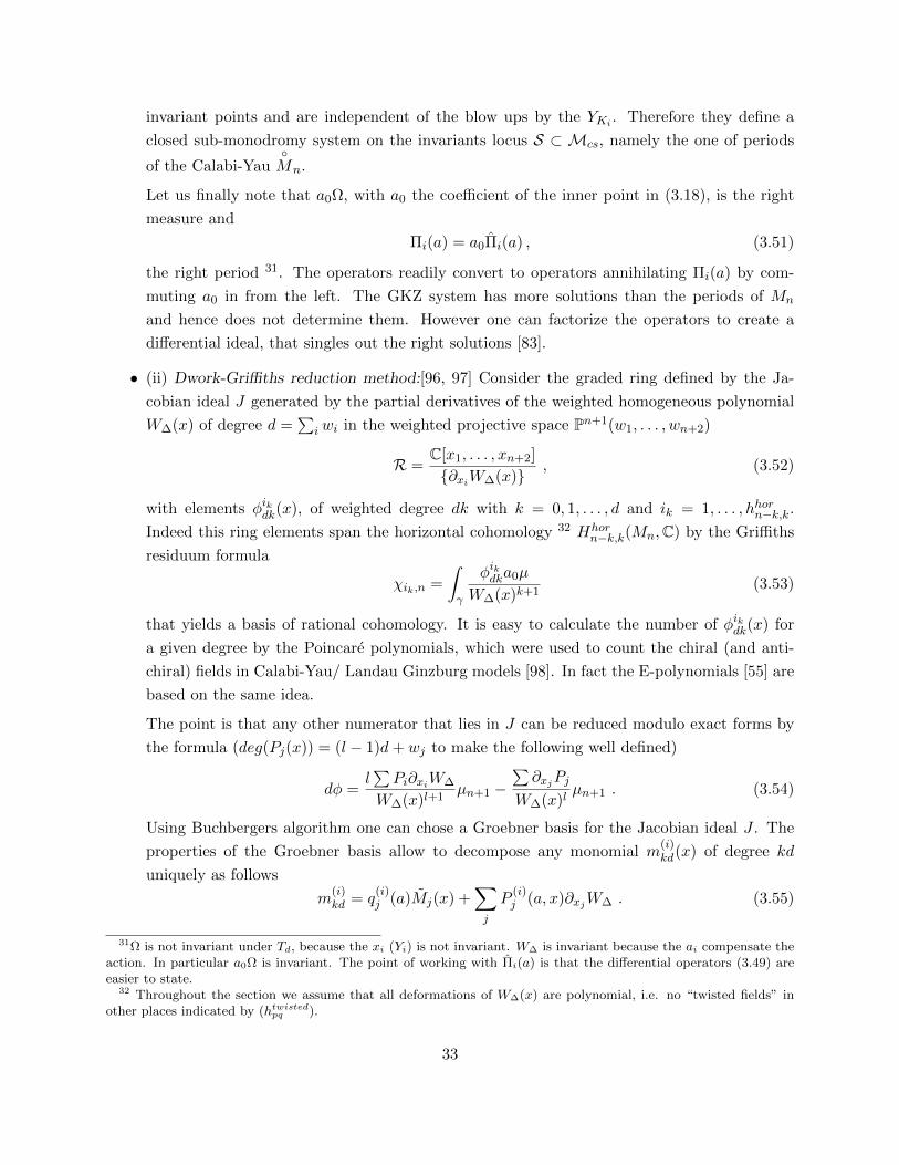
invariant points and are independent of the blow ups by the YKi . Therefore they define a
closed sub-monodromy system on the invariants locus S ⊂ Mcs, namely the one of periods
of the Calabi-YauMn.
Let us finally note that a0Ω, with a0 the coefficient of the inner point in (3.18), is the right
measure and
Πi(a) = a0Πi(a) , (3.51)
the right period 31. The operators readily convert to operators annihilating Πi(a) by com-
muting a0 in from the left. The GKZ system has more solutions than the periods of Mn
and hence does not determine them. However one can factorize the operators to create a
differential ideal, that singles out the right solutions [83].
• (ii) Dwork-Griffiths reduction method:[96, 97] Consider the graded ring defined by the Ja-
cobian ideal J generated by the partial derivatives of the weighted homogeneous polynomial
W∆(x) of degree d =∑
iwi in the weighted projective space Pn+1(w1, . . . , wn+2)
R =C[x1, . . . , xn+2]
∂xiW∆(x), (3.52)
with elements φikdk(x), of weighted degree dk with k = 0, 1, . . . , d and ik = 1, . . . , hhorn−k,k.
Indeed this ring elements span the horizontal cohomology 32 Hhorn−k,k(Mn,C) by the Griffiths
residuum formula
χik,n =
∫γ
φikdka0µ
W∆(x)k+1(3.53)
that yields a basis of rational cohomology. It is easy to calculate the number of φikdk(x) for
a given degree by the Poincare polynomials, which were used to count the chiral (and anti-
chiral) fields in Calabi-Yau/ Landau Ginzburg models [98]. In fact the E-polynomials [55] are
based on the same idea.
The point is that any other numerator that lies in J can be reduced modulo exact forms by
the formula (deg(Pj(x)) = (l − 1)d+ wj to make the following well defined)
dφ =l∑Pi∂xiW∆
W∆(x)l+1µn+1 −
∑∂xjPj
W∆(x)lµn+1 . (3.54)
Using Buchbergers algorithm one can chose a Groebner basis for the Jacobian ideal J . The
properties of the Groebner basis allow to decompose any monomial m(i)kd(x) of degree kd
uniquely as follows
m(i)kd = q
(i)j (a)Mj(x) +
∑j
P(i)j (a, x)∂xjW∆ . (3.55)
31Ω is not invariant under Td, because the xi (Yi) is not invariant. W∆ is invariant because the ai compensate theaction. In particular a0Ω is invariant. The point of working with Πi(a) is that the differential operators (3.49) areeasier to state.
32 Throughout the section we assume that all deformations of W∆(x) are polynomial, i.e. no “twisted fields” inother places indicated by (htwistedpq ).
33

Here Mj(x) are degree kd monomials in the multiplicative ringMR(Mj(x)) generated by the
Mj(x) in (3.18), q(i)j (a) is an unique rational function and the P
(i)j (a, x) are likewise uniquely
determined. In practice one uses (3.55, 3.54) as follows: One takes n+ 1 derivatives of (3.47)
w.r.t. to any of ai in (3.18). This produces an integrand Mi(x)/Wn+2∆ , whose numerator
is completely reducible by (3.55) to the last term on the r.h.s. The first term on the r.h.s
of (3.55) is zero as the ring R is empty at this degree. Using (3.54) one can reduce the
integrand, up to exact terms which do not affect the period integral, to sums of m(i)nd/W
(n+1)∆ .
Repeating the procedure reduces the n + 1th derivative to lower derivatives of (3.47) with
rational coefficients. This produces a differential operator for (3.47) as in the GKZ method.
Again the point is that this procedure closes into a closed sub-monodromy problem, if the
Newton polytope∆ is reflexive.
• (iii) The Mellin-Barnes integral method: At least for the toric cases this method is very similar
to the GGKZ method and relies on taking derivatives of the explicite Mellin-Barnes integral
representations [99],[100], which depend only on the l(α)-vectors in [99] and manipulating the
Mellin-Barnes integral. We discuss the formalism once the necessary background has been
developed in item (i) of section 3.10.2.
The formulas (3.47,3.52,3.53,3.54) have generalizations to the complete intersection case, see
e.g. [95] also (3.49) can be generalized [54, 95, 57], see also section 3.10.2.
The period vector Π(a) defined as Πi(a) =∫
Γ χi,n is annihilated by the connection
∇iΠ(a) = [∂ai + Cai(a)]Π(a) = 0 . (3.56)
Here χi,n spans a rational basis of the horizontal cohomology of Mn, see (3.53). The connection
(3.56) is obtained from IPf derived with methods (i) - (iii) by rewriting it as a system of first order
equations in the obvious way.
As we have seen in Calabi-Yau manifolds embedded in toric spaces with embedded polyhedra
as in (3.6.2) it is quite simple to conclude that there is a sub-monodromy problem on the invariant
subspace S. This is due to the special properties of generalized hypergeometric differential systems
with coefficients given in (3.50), which govern the periods of torically embedded Calabi-Yau spaces.
This methods does not exhaust all consistent sub monodromies problems of a given Calabi-Yau in a
toric ambient space as many sub-monodromy problems are of the Apery type [101][102] and at least
for the one moduli problems the vast majority of cases is of the Apery type. This is discussed for
the n = 1 case in [101] and for the n = 3, hn−1,1 = 1 case in [102] and references therein. They come
sometimes from much more exotic construction like from determinantal or Pfaffian CY-embeddings
in Grassmannians or Flag-manifolds or don’t have a known geometrical interpretation at all.
After introducing the concept of the flux super potential we give in section 3.11.3, based on the
integral structure of the monodromy, arguments that the idea of landscaping by fluxes applies to
these cases as well.
34

3.8 The calculable terms in the effective action
We review the simplest analytic quantities that depend on the complex moduli and can be calculated
from the topological string point of view and their interpretation in F-theory. All these can be
calculated in the B-model from the period integrals w.r.t. to an integral basis in homology or in
the A-model by localization w.r.t. to the torus action of the ambient space. The methods discussed
in section 3.7 yield linear differential equations for the periods, i.e. it remains to find those linear
combination in the solution space, which correspond to the integer basis.
3.8.1 Kahler potential, superpotential and Ray-Singer torsion
Our main interest is in the quantities which are involved in minimizing the flux superpotential.
Since all gauge symmetry enhancements are at high codimension in the generic moduli space of
the “clean sheet” Calabi-Yau manifolds one might conclude that F-theory predicts that there is
no unbroken gauge group at low energies. However as it was demonstrated in [31] for the case of
Seiberg-Witten gauge symmetry embedding in Calabi-Yau geometries a flux superpotential can at
least reduce this choice of o set of measure zero in the continuous moduli space to the discrete
choice of a flux, which in view of (3.15) might even be a discrete choice in a finite set of consistent
theories.
We are interested in F-theory super potentials on fourfolds and Type II super potentials on
threefolds and start with elements of the theory, which apply to the complex moduli spaces of
Calabi-Yau spaces of any dimensions namely the Weil-Petersson metric on the complex moduli
space Mcs, which determines the metric in front of the kinetic terms of the moduli fields. The
latter exist geometrically, because by the Tian-Todorov theorem the moduli space of Calabi-Yau
manifolds is unobstructed [103, 104]. Its tangent space are described by H1(Mn, TMn), which
can be identified with Hn−1,1(Mn) by contracting with Ωn. The metric on the complex moduli
space called Weil-Petersson metric is Kahler and the real Kahler potential is written in terms of
Ωn as [103, 104]
exp(−K(a, a)) = (−1)(n(n−1)/2)(2πi)n∫Mn
Ωn(a) ∧ Ωn(a) . (3.57)
As the no-where vanishing holomorphic Ωn form lives in a holomorphic line bundle L over Mcs
transforming as Ω(a) → ef(a)Ω(a), the Kahler form transforms in the Kahler line bundle with
Kahler transformations K(a, a) → K(a, a) − f(a) − f(a) so that e−K is a section of L ⊗ L. One
has natural covariant derivatives w.r.t. to the W-P metric connection and the Kahler connection
that act on sections Vj ∈ T ∗1,0Mcs ⊗ T ∗0,1Mcs ⊗ L⊗n ⊗ L⊗m as
DiVj = ∂iVj − ΓlijVl + nKiVj, DıVj = ∂ıVj − ΓlijVil +mKıVj, (3.58)
with Ki = ∂iK and Kı = ∂ıK. Griffiths transversality states that any combination ∇i1 . . .∇irof the application of the Gauss-Manin connection in the direction of complex moduli ai, i =
35

1, . . . ,dim(Mcs) to Ωn has the property
∇iΩn = ∇i1 . . .∇irΩ ∈ Fn−r , (3.59)
cff section 3.7. As a corollary to the T-T theorem χi = (∇i + Ki)Ω spans Hn,n−1(Mn). All
derivatives of Ω generate the primary horizontal subspace HnH(Mn). By consideration of Hodge
type and by (3.11) one gets
Q(∇iΩn,Ω) =
∫Mn
(∇i1 . . .∇irΩn) ∧ Ωn =
0 for 0 ≤ r < nCi1...in for r = n
(3.60)
The n-point coupling Ci1...in transforms as a section in L2 × Symn(T ∗Mcs). The underlying
field theory of the non-linear σ model has (2, 2) supersymmetry and can be twisted to the A and
the B model so that the chiral-chiral (c, c)-ring and the chiral-antichiral (c, a)-ring are identified
with Hp(Mn,∧qTMn) and HdR(Mn) respectively [105], where we focus on p = q = 1, . . . , n, but
only allow deformations for the p = q = 1 part of the cohomology 33 The holomorphic flux super
potential is given by
W =
∫Mn
Ωn(a) ∧Gn, (3.61)
where Gn has for fourfolds the properties discussed section 3.3, while for threefolds it is just integer
quantized in H3(M3,Z). The superpotential W obviously transforms in L. Generically one can
show using world-sheet arguments and mirror symmetry that Ω has to be viewed as the dilaton field
in topological string theory so that an amplitude, which can get genus χ = 2 − 2g − h instantons
corrections, transforms in Lχ [106], e.g. W can in fact be interpreted as a disk instanton potential.
As a consequence there is a natural L covariant derivative acting on W (z)
Di = ∂i + ∂iK , (3.62)
with ∂i = ∂ti , where ti is flat w.r.t. the Weil-Petersson connection.
To organize possible holomorphic terms related to the Griffiths Frobenius structure one can use
mirror symmetry and look at the index theorem that constrains the topological string A-model
amplitudes related to maps Φ : Σg → Cβ from the worldsheet Σg to curves Cβ ⊂ Wn in the class
β ∈ H2(Wn,Z) whose virtual dimension is
dimCMg,β(Wn) =
∫Cβ
c1(TWn)− (g − 1)(n− 3) . (3.63)
For Calabi-Yau n = 3-folds dimCMg,β(W3) = 0 and there is a rich Gromov-Witten theory on the
generic CY 3-fold in each genus. For g = 0 and n = 4 one has dimCM0,β(W4) = 1. To get an
enumerative problem one has to put the constraint Cβ ∩H4 6= 0, where H4 ∈ Hprim4 (W4,Z). The
33It was claimed in [3] that the more general deformations introduced by Kontsevich lead to residua calculationthat yields exact expressions for the Yukawa couplings.
36
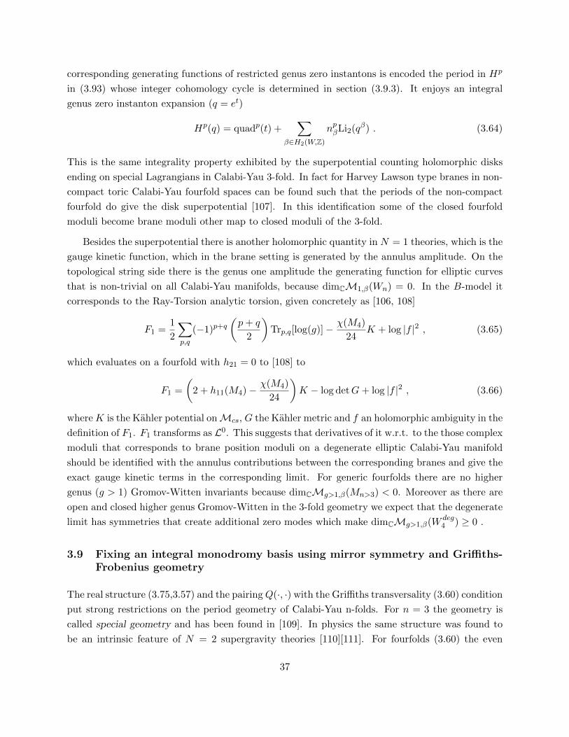
corresponding generating functions of restricted genus zero instantons is encoded the period in Hp
in (3.93) whose integer cohomology cycle is determined in section (3.9.3). It enjoys an integral
genus zero instanton expansion (q = et)
Hp(q) = quadp(t) +∑
β∈H2(W,Z)
npβLi2(qβ) . (3.64)
This is the same integrality property exhibited by the superpotential counting holomorphic disks
ending on special Lagrangians in Calabi-Yau 3-fold. In fact for Harvey Lawson type branes in non-
compact toric Calabi-Yau fourfold spaces can be found such that the periods of the non-compact
fourfold do give the disk superpotential [107]. In this identification some of the closed fourfold
moduli become brane moduli other map to closed moduli of the 3-fold.
Besides the superpotential there is another holomorphic quantity in N = 1 theories, which is the
gauge kinetic function, which in the brane setting is generated by the annulus amplitude. On the
topological string side there is the genus one amplitude the generating function for elliptic curves
that is non-trivial on all Calabi-Yau manifolds, because dimCM1,β(Wn) = 0. In the B-model it
corresponds to the Ray-Torsion analytic torsion, given concretely as [106, 108]
F1 =1
2
∑p,q
(−1)p+q(p+ q
2
)Trp,q[log(g)]− χ(M4)
24K + log |f |2 , (3.65)
which evaluates on a fourfold with h21 = 0 to [108] to
F1 =
(2 + h11(M4)− χ(M4)
24
)K − log detG+ log |f |2 , (3.66)
whereK is the Kahler potential onMcs, G the Kahler metric and f an holomorphic ambiguity in the
definition of F1. F1 transforms as L0. This suggests that derivatives of it w.r.t. to the those complex
moduli that corresponds to brane position moduli on a degenerate elliptic Calabi-Yau manifold
should be identified with the annulus contributions between the corresponding branes and give the
exact gauge kinetic terms in the corresponding limit. For generic fourfolds there are no higher
genus (g > 1) Gromov-Witten invariants because dimCMg>1,β(Mn>3) < 0. Moreover as there are
open and closed higher genus Gromov-Witten in the 3-fold geometry we expect that the degenerate
limit has symmetries that create additional zero modes which make dimCMg>1,β(W deg4 ) ≥ 0 .
3.9 Fixing an integral monodromy basis using mirror symmetry and Griffiths-Frobenius geometry
The real structure (3.75,3.57) and the pairingQ(·, ·) with the Griffiths transversality (3.60) condition
put strong restrictions on the period geometry of Calabi-Yau n-folds. For n = 3 the geometry is
called special geometry and has been found in [109]. In physics the same structure was found to
be an intrinsic feature of N = 2 supergravity theories [110][111]. For fourfolds (3.60) the even
37

bilinear form Q(·, ·) gives algebraic as well differential relations among the periods. The Frobenius
structure is more interesting as its maximal grade is n, which implies that for n ≥ 4 it allows for
various types of three point functions and non-trivial associativity constraints. In addition the real
structure (3.57) gives non-holomorphic relations between the two types of couplings and the metric
structure. Even though (F-theory) compactifications on 4-folds lead to N = 1 supergravity and the
structure is in part similarly realized in open string compactifications with N = 1 supergravity, it is
not intrinsic in N = 1 supergravity. We will refer to the structure therefore as Griffiths-Frobenius
geometry with the understanding that it is N = 2 special geometry for compactifications on M3.
Finding the Griffiths-Frobenius geometry in 4d N = 1 physics on the other hand would be a hint
for string theory.
Combined with mirror symmetry, which maps the Griffiths-Frobenius geometry on the (c, c)
B-model ring to the one on the (a, c) A-model ring, the constraints turn out to be strong enough to
find an integral monodromy basis. For CY 3-folds with one parameter this was done in [99] [71][72]
and for arbitrary number of parameters in [95]. We give a result oriented review of this in section
3.9.2, where we stress the elements of the theory that apply to any dimension.
Even though genus zero instantons for one parameter families of Calabi-Yau spaces in various
dimensions have been calculated in [112] and for multi parameter fourfolds in [113, 1] and even
genus one instantons and their multi covering formula of the genus zero curves has been found and
confirmed in several multi parameter fourfolds [108] the integral monodromy basis on the primary
horizontal subspace of H4(M4) has not been determined. The structures discussed partly in [112]
and in [1, 113] are a prerequisite to determine this basis and will be discussed and extended in
the section 3.9.1. Expressions for the Kahlerpotential the large complex structure points can be
obtained from the sphere partition function [114, 115][116][117].
In section 3.9.3 we use the structures described above to find this basis. We exemplify this first
with the sixtic in P5 and eight other examples and generalize this to the most general constructions
of fourfolds using the hemi-sphere partition function in section 3.10.2. Once this integral basis
has been determined one can also set up the tt∗ structure and study it at those degenerations of
fourfolds that are interesting for F-theory.
3.9.1 The Frobenius algebra and the tt∗ structure
A Frobenius algebra has the following elements. It is a graded vector space A = ⊕A(i), i ≥ 0 with
a symmetric non-degenerate bilinear form η and a cubic form
C(i,j,k) : A(i) ⊗A(j) ⊗A(j) → C. (3.67)
Here is the list of defining properties:
• FAs) Symmetry: C(i,j,k)abc = C
(σ(i,j,k))σ(abc) under any permutation of indices.
38

• FAd) Degree:34 C(i,j,k) = 0 unless i+ j + k = n.
• FAu) Unit: C(0,i)1ab = η
(i)ab .
• FAnd) Non-degeneracy: C(1,j) is non-degenerate in the second slot.
• FAa) Associativity: C(i,j)abp η
pq(n−i−j)C
(i+j,k)qcd = C
(i,k)acq η
qp(n−i−k)C
(i+k,j)pbd .
Here the latin indices a, b, c, . . . refer to a choice of basis A(i)a , a = 1, . . . ,dim(A(i)) of A(i). The
above defines a commutative algebra as follows
A(i)a · A
(j)b = C
(i,j)abq η
qp(i+j)A
(i+j)p = C
(i,j)pab A(i+j)
p . (3.68)
These structures are intrinsic to the (c, c)- and (a, c)-rings of the worldsheet (2, 2) superconformal
theory. The charges of the U(1)A and U(1)V currents in the (2, 2) supersymmetry algebra define
the grading in the (c, c)- and the (a, c) rings respectively and the rest of the Frobenius structure
follows from the axioms of conformal field theory and the closing of the rings up to QB, QA exact
terms, see [118]. Note that in families of Frobenius algebras η(p)ab is a constant topological pairing,
while the general C(i,j)abc (t) varies with the deformation parameter.
In the B-model the (c, c) ring is identified for fixed complex structure with the elements B(p,q)a
in Hp(M,∧qTM). We consider only those elements which are mapped by contraction with Ω to
elements B(p) = Ω(B) in Hnprim(Mn), i.e. in particular p = q. The Hodge type for this complex
structure, which can be taken at the point of maximal unipotent monodromy, defines the grading,
so that one gets
C(p,q)abc = Q(Ω(B(p)
a ∧B(q)b ∧B
(n−p−q)c ),Ω) , (3.69)
which depends also on the Kahlergauge of Ω. For complex families, i.e. deformations w.r.t. elements
with (p = q = 1), the grade of B(p) is encoded in the filtration parameter of Fn−p and we give a
covariant definition of (3.69) below.
The (a, c) ring is mapped to the quantum cohomology extension of H∗deRham. On the vertical
cohomology in Hp,p(Mn) the grading of the A-model is simply identified with the form degree. We
allow again only the complexified Kahler deformation family w.r.t. to elements with p = 1. These
deformation families of rings are pairwise identified by mirror symmetry on M and W and at the
point of maximal unipotent monodromy the gradings can be matched using the monodromy weight
filtration. This gives important information about the basis of the cohomology and homology
groups in Hnprim(Mn).
One can chose a basis AI(p) of the homology Hn(Mn,Z) and a dual one α(p)I for cohomology of
the primary horizontal subspace so that∫AI
(p)
α(q)J = δIJδ
qp,
∫Mn
α(q)I ∧ α
(p)J =
0 if p+ q > n,
η(q)IJ if p+ q = n .
(3.70)
34Because of this property the last index indicating the degree dropped in the following.
39
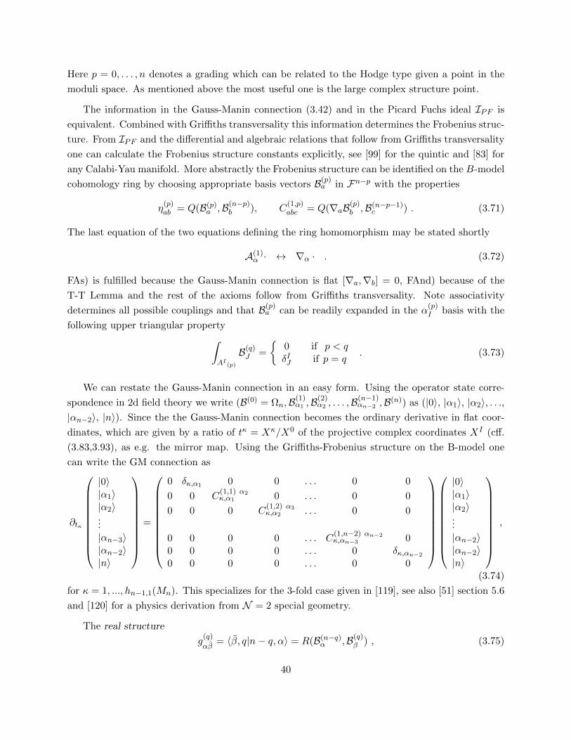
Here p = 0, . . . , n denotes a grading which can be related to the Hodge type given a point in the
moduli space. As mentioned above the most useful one is the large complex structure point.
The information in the Gauss-Manin connection (3.42) and in the Picard Fuchs ideal IPF is
equivalent. Combined with Griffiths transversality this information determines the Frobenius struc-
ture. From IPF and the differential and algebraic relations that follow from Griffiths transversality
one can calculate the Frobenius structure constants explicitly, see [99] for the quintic and [83] for
any Calabi-Yau manifold. More abstractly the Frobenius structure can be identified on the B-model
cohomology ring by choosing appropriate basis vectors B(p)a in Fn−p with the properties
η(p)ab = Q(B(p)
a ,B(n−p)b ), C
(1,p)abc = Q(∇aB(p)
b ,B(n−p−1)c ) . (3.71)
The last equation of the two equations defining the ring homomorphism may be stated shortly
A(1)α · ↔ ∇α · . (3.72)
FAs) is fulfilled because the Gauss-Manin connection is flat [∇a,∇b] = 0, FAnd) because of the
T-T Lemma and the rest of the axioms follow from Griffiths transversality. Note associativity
determines all possible couplings and that B(p)a can be readily expanded in the α
(p)I basis with the
following upper triangular property∫AI (p)
B(q)J =
0 if p < qδIJ if p = q
. (3.73)
We can restate the Gauss-Manin connection in an easy form. Using the operator state corre-
spondence in 2d field theory we write (B(0) = Ωn,B(1)α1 ,B
(2)α2 , . . . ,B
(n−1)αn−2 ,B(n)) as (|0〉, |α1〉, |α2〉, . . .,
|αn−2〉, |n〉). Since the the Gauss-Manin connection becomes the ordinary derivative in flat coor-
dinates, which are given by a ratio of tκ = Xκ/X0 of the projective complex coordinates XI (cff.
(3.83,3.93), as e.g. the mirror map. Using the Griffiths-Frobenius structure on the B-model one
can write the GM connection as
∂tκ
|0〉|α1〉|α2〉...|αn−3〉|αn−2〉|n〉
=
0 δκ,α1 0 0 . . . 0 0
0 0 C(1,1) α2κ,α1 0 . . . 0 0
0 0 0 C(1,2) α3κ,α2 . . . 0 0
0 0 0 0 . . . C(1,n−2) αn−2κ,αn−3 0
0 0 0 0 . . . 0 δκ,αn−2
0 0 0 0 . . . 0 0
|0〉|α1〉|α2〉...|αn−2〉|αn−2〉|n〉
,
(3.74)
for κ = 1, ..., hn−1,1(Mn). This specializes for the 3-fold case given in [119], see also [51] section 5.6
and [120] for a physics derivation from N = 2 special geometry.
The real structure
g(q)
αβ= 〈β, q|n− q, α〉 = R(B(n−q)
α ,B(q)β ) , (3.75)
40

and the worldsheet parity operation
〈α, q| = 〈β|M (q)βα , (3.76)
which fulfills the worldsheet CPT constraints MM∗ = 1, extend the Griffiths-Frobenius package
on the mixed Hodge structure to the tt∗- structure [106].
In particular one can chose the basis B(p)α compatible with the real structure, i.e.
B(p)α = B(n−p)
α . (3.77)
The degree one elements are the well known tangents vectors to the complex deformation space of
Tian and Todorov
B(1)α = DαΩ, B(1)
α = DαΩ . (3.78)
Note that g(q)
αβis the Zamolodichkov metric, gi is related to the Weil-Petersson metric Gi by
g(1)i = e−KGi = 〈0|0〉Gi and has blockform w.r.t. to the grading. The higher degree operators are
given for p = 2, . . . , bn2 c by
Bpα = D(p)α Ω, B(p)
α = D(p)α Ω, (3.79)
with D(p)α = 1
p!κα;i1,...,ipDi1 . . . Dip . These operators are closely related to the Frobenius operator
D(p)(ρ) and as the latter determined at the point of maximal unipotent monodromy from the symbol
of the Picard-Fuchs differential ideal IPF on Mn as in (3.143) or equivalently from the information
in the Chow ring of Wn. In order to fix them completely in the n > 3 cases one has to construct
the integer basis, which we do in sections 3.9.3, with the generalizations in sections 3.10,3.10.2.
Note that the metric connection to gi is Kahler, i.e. pure γkij = g lk∂jgjl, γkı = gkl∂ıgl and
defines metric connections di = ∂i − γi and dı = ∂ı − γı. The tt∗ connection is defined as
∇i = di + Ci , ∇i = d + Cı , (3.80)
C denotes the complex conjugated Frobenius structure constants, they have pure holomorphic
or anti-holomorphic indices, which are raised and lowered with the constant topological pairing
ηij = ηı. All expressions inherit the grading from the Frobenius algebra, which we suppress in this
paragraph. One has the tt∗ relations of Cecotti and Vafa, see [121] for a review for CY-3 folds,
[di, dj ] = [dı, d] = [di, Cı] = [dı, Ci] = 0,
[di, Cj ] = [dj , Ci], [dı, C] = [d, Cı],
[di, d] = −[Cj , Cı], hence [∇i,∇j ] = [∇ı,∇] = [∇i,∇] = 0 .
(3.81)
The connection ∇i is the Gauss-Manin connection and the last equation promotes that structure
to the flat tt∗ connection.
Mathematically the tt∗-structure is related to the TERP-structure, see review of Hertling and
Sabbah [122], and the non-commutative Hodge structure [123]. It was in the latter context that
the Γ classes were found in [123], that we use in section 3.10 to confirm the integral basis that we
determine in section 3.9.3.
41

3.9.2 Integral basis for the middle homology of Calabi-Yau threefolds
For n = 3 and more generally n odd Hn(Mn,Z) is primitive, η is antisymmetric and one can chose a
symplectic basis αI , βI , in Hn(Mn,Z) and a dual one AI , BI , I = 0, . . . , h = bn/2−1 in Hn(Mn,Z)
with a symplectic pairing
Σ =
(0 1k×k
−1k×k 0
). (3.82)
Then Ω can be expanded in the symplectic basis of Hn(Mn,Z) in terms of the period vector
Π(a) = (XI =∫AI Ω(a), FI =
∫BI
Ω(a))T over the symplectic basis of Hn(Mn,Z) as
Ω = XIαI − FIβI , (3.83)
and the Kahler potential becomes
e−K = iΠ†(a)ΣΠ(a), (3.84)
while the superpotential is
W = qIXI − pIFI , (3.85)
where qI and pI in Z are electric and magnetic charges. Using (3.60) one derives for n = 3 the
existence of special geometry [124] and in particular an holomorphic prepotential F , homogeneous
degree two in the XI periods with FI = ∂F∂XI , which determines the periods, the couplings Cijk, as
well as the Kahler potential, hence the name. Based on the seminal work of [99] and the mirror
symmetry conjecture it was pointed out in [95] how to fix in general an integer symplectic basis for
the periods at the large complex structure point from the topological data of the mirror manifold
Wn35 where i, j, k = 1, . . . , h
F = −C0ijkX
iXjXk
3!X0+ nij
XiXj
2+ ciX
iX0 − i χζ(3)
2(2π)3(X0)2 + (X0)2f(q)
= (X0)2F = (X0)2
[−Cijkt
itjtk
3!+ nij
titj
2+ cAt
A − i χζ(3)
2(2π)3+ f(q)
]. (3.86)
It defines an integral basis for the periods at the large complex structure points given by
Πlcs =
X0
Xi
F0
Fi
= X0
1ti
2F − ti∂iF∂F∂ti
= X0
1ti
C0ijk
3! titjtk + cit
i − iχζ(3)(2π)3 + f(q)
−C0ijk
2 titj + nijtj + ci + ∂if(q)
. (3.87)
Here we defined the mirror map ti(a) as
ti(a) =Xi(a)
X0(a)=
1
2πi
(log(zi) + Σi(z)
), i = 1, . . . , hn−1,1 . (3.88)
35This large volume point might not be unique. There are as many such points as there different Calabi-Yautriangulations of ∆∗, and hence different Mori vectors. Each defines by (3.30) a large volume point, which correspondto different phases of Wn.
42

Note that ti has in the A-model, the interpretation of a complexified area ti =∫Ci(J+iB2), where J
is the Kahler form and B2 is Neveu-Schwarz two form on Wn. The map ti(a) can be made explicit
at the large complex structure point using
X0(a) = ω0(z(a), ρ)|ρ=0, (3.89)
with ω0(z(a), ρ) defined in (3.50) and z(a) defined in (3.30) as well as
Xi =1
2πi∂ρiω0(z(a), ρ)|ρ=0 . (3.90)
This is the first step in the construction of solutions by the Frobenius method, which relies on
the fact that certain differential operators, the Frobenius operators D(k)(ρ) in ρ with constant
coefficients 36 of degree k = 1, . . . , n commute
[Di(z),D(k)(ρ)]|ρ=0 = 0, (3.91)
on the solution space with the operators in IPF . IPF determines the structure constants of the
Frobenius algebra that appears in the periods. This fact determines the D(k)(ρ) [83]. In particular
due to FAnd) (3.91) holds for all operators of degree k = 1, which yields (3.90) in any dimension.
Another universal solution is 37
D(n)(ρ)ω0(z(a), ρ)|ρ=0 =C0i1,...,in
n!(2πi)n∂ρi1 · · · ∂ρinω0(z(a), ρ)|ρ=0 , (3.92)
where the C0i1,...,in
=∫Wn
Ji1 ∧ . . . ∧ Jin ≥ 0 are the classical intersection numbers and Ji are
(1, 1)-forms in H2(W3,Z), which span the Kahlercone. The solution (3.92) has in the A-model the
interpretation of a 2n-volume. F0 =∫A(n) Ω contains (3.92) and lower logarithmic solutions. In the
homological mirror symmetry interpretation F0 is the central charge of the D2n brane, which corre-
spond to the structure sheaf on W . The lower logarithmic solutions are the K-theoretic corrections
due to induced lower brane charges. For n = 3 one has ci = 124
∫W3
c2∧Ji and nij =∫W3
i∗c1(Di)∧Jj .
Special geometry implies that D(2)k (ρ) =
C0ijk
3!(2πi)2∂ρi∂ρjω0(z(a), ρ)|ρ=0, h = 1, . . . , h21 are also solu-
tions. The q expansion of FI around the large volume is the worldsheet instanton expansion on
W3. Note that the explicit form of f(q) is completely determined by (3.50) and its derivatives with
respect to ρ, whose precise structure is fixed by the ti polynomials. The methods fixes the period
vector in an integer basis near the large complex structure point with a finite radius of convergence
and hence everywhere else in Mcs by analytic continuation.
Beside F0 =∫A(n) Ω, the other universal solution X0 =
∫A(0) Ω is the D0-brane central charge,
which corresponds in the A-model to the sky-scraper sheaf on W . The cycle A(n) has the topology
36Which are given by the classical intersection of the A model, see below.37Here we sum over equal indices. We denote by C0
i1,...,in the classical intersections, which are a valid approximationonly at the large radius point, while Ci1,...,in are the intersections in quantum cohomology, which are exact expressionsthroughout the complexified Kahler- or complex moduli space.
43

of an Sn sphere, which is the one that vanishes at the generic conifold divisor compare (3.164) and
is in the class of the base of Strominger-Yau-Zaslow fibration, while A(0) has the topology of a Tn
and is in the class of the SYZ torus fibre. According to SYZ mirror symmetry is T -duality on Tn
and maps Type II A/B on Mn to Type II B/A on Wn for n odd and Type II A/B on Wn for n
even.
An explanation of the ζ(k) terms from the Frobenius method was given in [95]. In particular
the term i χζ(3)2(2π)3 comes from the third derivative of the Γ-function in (3.50) due to D(3). This logic
applies also to the B-model in higher dimensional Calabi-Yau space. Recently it has been realized
in the context of homological mirror symmetry [125, 123, 126] that these subleading terms can be
obtained by modifying the Chern-Character map in the K-theory group of the A-model by the Γ
classes. In section 3.10.1 we summarize this formalism as a check of the integral monodromy basis
determined that we determine on the B-model side in the next section.
3.9.3 Integral basis for the primitive horizontal homology of fourfolds
If n is even then the primitive part of HnH(Mn) that is accessible to the analysis by period integrals
on Mn is a subspace of Hn(Mn). By mirror symmetry the vertical subspace HV (Mn) is accessible
to the analysis by period integrals on Wn. Often in the toric context the intersection of these spaces
gives all of Hn(Mn). The techniques that we develop below allow to find the integral monodromy
basis for both cohomologies. These integer structures are necessary to make these cohomology
elements well defined on the corresponding deformation family. By the dimensional argument in
viii) of section 3.3 it is in general not possible to find an integral element in H∗(Mn,Z) that lies
entirely in HnH(Mn) or Hn
V (Mn) 38. In any case the elements might be rational in H∗(Mn,Z), but
they can be added to an integer basis of H∗(Mn,Z) with coefficients one that can be reconstructed
from the lattice structure and the monodromy information.
The two subspaces govern the vacuum structure of the complex moduli and the Kahler moduli
by the F -term superpotentials respectively. To actually calculate those F -terms that restrict the
complex moduli from the fluxes on the primitive horizontal space on M4 we determine now the
integer monodromy basis that allows to evaluate the formulas (2.1, 3.57,3.61) explicitly.
This requires to delve deeper into the structure of periods on fourfolds discussed in section 3.9.1.
We expand the (4, 0) form Ω in terms of the basis α(p)I of the primary horizontal subspace as
Ω = X0α(0) +Xiα(1)i +Hpα
(2)p + Fiα(3)i + F0α
(4) , (3.93)
where i = 1, . . . , h = h3,1, p = 1, . . . , k = hprim2,2 . Due to the grading the bilinear form Q on
38The argument does not exclude the possibility to find such a splitting over Z/2. Even if the dimensional argumentdoes not forbid a separation, it is still unlikely to occur, because it is physically expected for N = 1 theories that theKahler and complex moduli sector do couple and the available concrete discussion of conditions on fluxes is still veryincomplete.
44

Hprim4 (M4), has the form
Q∗(Γ,Γ) = ΓαηαβΓβ = ΓT
∗ ∗ ∗ ∗ 1
∗ ∗ ∗ η(1)h×h
∗ ∗ η(2)k×k
∗ (η(1))Th×h1
Γ . (3.94)
We claim that with a GL(h4,Z) transformation we can eliminate the ∗ entries and bring Q in a
block anti-diagonal form. Instead of special geometry Griffiths transversality implies
2XF +H2 = 0, (η(1)F )i +X∂iF +H∂iH = 0, X∂i∂jF +H∂i∂jH = 0,X∂i∂j∂kF +H∂i∂j∂kH = 0, X∂i∂j∂k∂lF +H∂i∂j∂k∂lH = C ′ijkl, (3.95)
where we used a vector notation for the periods X,H,F = ∫
ΓiΩ and the pairing on the periods
induced from (3.94) in the block anti-diagonal form.
Analogously to section 4.2 in [83] (3.95) and the differential equations derived from (3.49) can
be used to obtain the Ci1,...,ir and match the Frobenius structure as [113, 1]
Cijkl = C(1,1,2)ijp ηpq2 C
(2,1,1)pkl = ∂i∂jH∂k∂lH . (3.96)
We will now show how this structure and the observations discussed in section 3.11.2 can be used
to fix an integral basis for the primitive homology of a fourfold. Let us treat the sextic in P5 and
develop the general picture along the way. After dividing by Z46 acting as xi → exp(2πir
(l)i )xi with
r(1) = 16(1, 5, 0, 0, 0, 0), r(2) = 1
6(1, 0, 5, 0, 0, 0), r(3) = 16(1, 0, 0, 5, 0, 0) and r(4) = 1
6(1, 0, 0, 0, 5, 0) one
gets the invariant sextic constraints defined in P5/Z46 as
W∆inv = P =6∑i=1
aix6i − a0
6∏i=1
xi. (3.97)
The same combinatorics is encoded in the vertices of ∆∗ spanned by νi = ei, i = 1, . . . , 5 and
ν6 = −∑5
i=1 ei so that P = W∆∗ and l(1) = (−6; 1, 1, 1, 1, 1, 1) and the Picard-Fuchs follows
from (3.49) to be in the large complex structure variable (3.30) given as (3.165) with k = 6.
The ai, i = 1, . . . , 6 are gauged to 1 by the Tn+1 × C action and we call a0 simply a in the
following. The complex moduli space is parametrized by z = 1/a6 and can be compactified to
Mcs = P1 \z = 0, z = 166 , 1/z = 0, where the critical points are the large complex structure point
z = 0, the conifold point z = 166 and an Z6 orbifold point. The mirror39 has hprim
4 (W4) = 5 and
the five solutions of (3.165) corresponds to the integrals over the five dual 4-cycles. Using mirror
39According to [49] χ = 2160 moreover from Thm. 4.3.7 of [49] (n in [49] is the dimension of P∆) one hash31(M4) = 426, h11(M4) = 1. Hence h21(M4) = 0 from (3.7), moreover from section 3.3 one gets σ(H22) = 1752,where the primitive part contributes 1751 and the vertical part 1 to H+(M4). Hence Hprim
22 (W4) = 1.
45
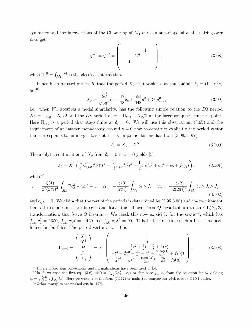
symmetry and the intersections of the Chow ring of M4 one can anti-diagonalize the pairing over
Z to get
η−1 = ηαβ =
1
1C0
11
, (3.98)
where C0 =∫M4
J4 is the classical intersection.
It has been pointed out in [5] that the period Xν that vanishes at the conifold δc = (1 − 66z)
as 40
Xν =2δ
32c√
3π2(1 +
17
18δc +
551
648δ2c +O(δ3
c )), (3.99)
i.e. when Wn acquires a nodal singularity, has the following simple relation to the D0 period
X0 = Πreg + Xν/2 and the D8 period F0 = −Πreg + Xν/2 at the large complex structure point.
Here Πreg is a period that stays finite at δc = 0. We will use this observation, (3.95) and the
requirement of an integer monodromy around z = 0 now to construct explicitly the period vector
that corresponds to an integer basis at z = 0. In particular one has from (3.98,3.167)
F0 = Xν −X0 . (3.100)
The analytic continuation of Xν from δc = 0 to z = 0 yields [5]
F0 = X0
(1
4!C0ijklt
itjtltk +1
3!cijkt
itjtk +1
2cijt
itj + citi + c0 + f0(q)
), (3.101)
where41
c0 =ζ(4)
22(2πi)4
∫M4
(7c22 − 4c4)− 1, c1 = − ζ(3)
(2πi)3
∫M4
c3 ∧ Ji, cij = − ζ(2)
2(2πi)2
∫M4
c2 ∧ Ji ∧ Jj ,
(3.102)
and cijk = 0. We claim that the rest of the periods is determined by (3.95,3.96) and the requirement
that all monodromies are integer and leave the bilinear form Q invariant up to an GL(h4,Z)
transformation, that leave Q invariant. We check this now explicitly for the sextic42, which has∫M4
c22 = 1350,
∫M4
c3J = −420 and∫M4
c2J2 = 90. This is the first time such a basis has been
found for fourfolds. The period vector at z = 0 is
Πz=0 =
X0
X1
HF1
F0
= X0
1t
−12 t
2 + 12 t+ 5
8 + h(q)
−t3 + 32 t
2 − 34 t−
158 + 105iζ(3)
2π3 + f1(q)14 t
4 + 158 t
2 − 105iζ(3)2π3 t− 75
64 + f2(q)
. (3.103)
40Different and sign conventions and normalizations have been used in [5].41In [5] we used the first eq. (3.6) 1440 =
∫W4
(3c22 − c4) to eliminate∫W4
c4 from the equation for c0 yielding
c0 = ζ(4)
22(2πi)4
∫M4
5c22. Here we write it in the form (3.102) to make the comparison with section 3.10.1 easier.42Other examples are worked out in [127].
46
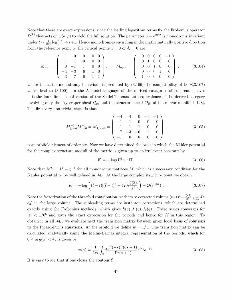
Note that these are exact expressions, since the leading logarithm terms fix the Frobenius operator
D(k)i that acts on ω(a, ρ) to yield the full solution. The parameter q = e2πit is monodromy invariant
under t ∼ 12πi log(z)→ t+1. Hence monodromies encircling in the mathematically positive direction
from the reference point p0 the critical points z = 0 or δc = 0 are
Mz=0 =
1 0 0 0 01 1 0 0 00 −1 1 0 0−4 −3 6 1 0
3 7 −6 −1 1
, Mδc=0 =
0 0 0 0 −10 1 0 0 00 0 1 0 00 0 0 1 0−1 0 0 0 0
, (3.104)
where the latter monodromy behaviour is predicted by (3.166) the compatibility of (3.98,3.167)
which lead to (3.100). In the A-model language of the derived categories of coherent sheaves
it is the four dimensional version of the Seidel-Thomas auto equivalence of the derived category
involving only the skyscraper sheaf Qpt and the structure sheaf OW of the mirror manifold [128].
The first very non trivial check is that
M−1δc=0M
−1z=0 = M1/z=0 =
−4 4 0 −1 −1−1 1 0 0 0−1 1 1 0 0
7 −3 −6 1 0−1 0 0 0 0
, (3.105)
is an orbifold element of order six. Now we have determined the basis in which the Kahler potential
for the complex structure moduli of the metric is given up to an irrelevant constant by
K = − log(Π†η−1Π). (3.106)
Note that M tη−1M = η−1 for all monodromy matrices M , which is a necessary condition for the
Kahler potential to be well defined in Mc. At the large complex structure point we obtain
K = − log
((t− t)[(t− t)3 + 420i
ζ(3)
π3]
)+O(e2πit) . (3.107)
Note the factorization of the threefold contribution, with its α′ corrected volume (t−t)3− iζ(3)π3
∫W4
J∧c3) in the large volume. The subleading terms are instanton corrections, which are determined
exactly using the Frobenius methods, which gives h(q), f1(q), f2(q). These series converges for
|z| < 1/66 and gives the exact expression for the periods and hence for K in this region. To
obtain it in all Mcs we evaluate next the transition matrix between given local basis of solutions
to the Picard-Fuchs equations. At the orbifold we define w = 1/z. The transition matrix can be
calculated analytically using the Mellin-Barnes integral representation of the periods, which for
0 ≤ arg(a) < π3 , is given by
$(a) =1
2πi
∫Cds
Γ(−s)Γ(6s+ 1)
Γ5(s+ 1)eiπsa−6s . (3.108)
It is easy to see that if one closes the contour C
47

• a.) along a = −ε to the right to enclose all the poles at s ∈ N one gets $(a) = X0(z),
convergent for |z| < 166 ,
• b.) while if one closes it to left to enclose all the poles at s = −l/6 with l ∈ N+ one gets a
solution at the orbifold convergent for |a| < 6
$0(a) = −1
6
∑m=1
eπim5/6 Γ(m6
)Γ(m)Γ5
(1− m
6
)am . (3.109)
The other four solutions at the orbifold are given by $i(a) = $0(βia), i = 1, . . . , 4 with β = e2πi6 .
In the $i(a), i = 0, . . . , 4 basis of solutions the monodromy upon a→ βa is obviously given by
M1/z=0 =
0 1 0 0 00 0 1 0 00 0 0 1 00 0 0 0 1−1 −1 −1 −1 −1
. (3.110)
To analytically continue the other four solutions to z = 0 one notes that
$k(a) = − 1
6(2πi)5
5∑p=1
βkp(βp − 1)$(a), (3.111)
where
$k(a) = −∫C
ds
e2πsi − 1
Γ6(s+ s
6
)Γ(6s+ k)
a6s+k , (3.112)
with the contour of type b.). Choosing the contour along the path described as in a.) a slightly
tedious calculation allows to match the logarithm of z and get the transition matrix Πz=0 =
m($0, $1, $2, $3, $4)T by comparing with (3.103) as
m =
1 0 0 0 0
−16
23
12
13
16
14
23
14 0 − 1
1213 −4
3 1 43
23
0 −1 0 0 0
. (3.113)
It is a nontrivial check that M1/z=0 = m−1M1/z=0m. It is harder to determine completely the
transition matrix from the large complex structure point to the conifold exactly Πz=0 = n(1 −1
3888δ4c +O(δ5
c ), δc + 198119440δ
4c +O(δ5
c ), δ2c − 41
48δ4c +O(δ5
c ), δ3c + 125
72 δ4c +O(δ5
c ), Xν) . We reduced the
50 real constants of n to 14 which we determined numerically.
n =
a b c d 1
ia1 ib1 ic1 id1 0
a1 + ia22 b1 + i b22 c1 + i c22 d1 + id2
2 0
−3a2 + ia3 −3b2 + ib3 −3c2 + ic3 −3d2 + id3 0
−a −b −c −d 1
. (3.114)
48
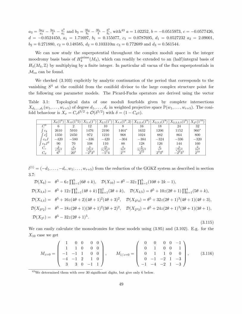
a3 = 3a2a1− 3a1
4 −a2
a1and b3 = 3b2
b1− 3b1
4 −b2
b1, with43 a = 1.02252, b = −0.0515973, c = −0.0577426,
d = −0.0524450, a1 = 1.71697, b1 = 0.155077, c1 = 0.0787695, d1 = 0.0527232 a2 = 2.09001,
b2 = 0.271880, c2 = 0.148585, d2 = 0.103310m c3 = 0.772689 and d3 = 0.561544.
We can now study the superpotential throughout the complex moduli space in the integer
moodromy basis basis of Hprime4 (M4), which can readily be extended to an (half)integral basis of
H4(M4,Z) by multiplying by a finite integer. In particular all vacua of the flux superpotentials in
Mcs can be found.
We checked (3.103) explicitly by analytic continuation of the period that corresponds to the
vanishing S4 at the conifold from the conifold divisor to the large complex structure point for
the following one parameter models. The Picard-Fuchs operators are derived using the vector
Table 3.1: Topological data of one moduli fourfolds given by complete intersectionsXd1,...,dr(w1, . . . , wr+5) of degree d1, . . . , dr in weighted projective space P(w1, . . . , wr+5). The coni-fold behaviour is Xν = Ccδ
3/2 +O(δ5/2) with δ = (1− Cdz).
X6(16) X10(155) X3,4(17) X2,5(17) X4,4(16, 2) X2,2,4(18) X2,3,3(18) X2,2,2,3(19) X25(110)
C0 6 2 12 10 8 16 18 24 32∫c4 2610 5910 1476 2190 1464∗ 1632 1206 1152 960∗∫c22 1350 2450 972 1210 968 1024 882 864 800∫c3J −420 −580 −336 −420 −304 −384 −324 −336 −320∫c2J
2 90 70 108 110 88 128 126 144 160Cc
2√3π2
23π2
4√6π2
10
3√
5π24
3π28
3√
2π22π2
4√3π2
23π2
Cd 66 205 −2833 −554 214 212 2436 −2633 210
l(1) = (−d1, . . . ,−dr, w1; . . . , wr+5) from the reduction of the GGKZ system as described in section
3.7:
D(X6) = θ5 − 6z∏5k=1(6θ + k), D(X10) = θ5 − 32z
∏5k=1(10θ + 2k − 1),
D(X3,4) = θ5 + 12z∏3k=1(4θ + k)
∏2k=1(3θ + k), D(X2,5) = θ5 + 10z(2θ + 1)
∏4k=1(5θ + k),
D(X4,4) = θ5 + 16z(4θ + 2)(4θ + 1)2(4θ + 3)2, D(X224) = θ5 + 32z(2θ + 1)3(4θ + 1)(4θ + 3),
D(X322) = θ5 − 18z(2θ + 1)(3θ + 1)2(3θ + 2)2, D(X233) = θ5 + 24z(2θ + 1)3(3θ + 1)(3θ + 1),
D(X25) = θ5 − 32z(2θ + 1)5.(3.115)
We can easily calculate the monodromies for these models using (3.95) and (3.102). E.g. for the
X10 case we get
Mz=0 =
1 0 0 0 01 1 0 0 0−1 −1 1 0 0−4 −1 2 1 0
3 3 0 −1 1
, M1/z=0 =
0 0 0 0 −10 1 0 0 10 1 1 0 00 −1 −2 1 −3−1 −4 −2 1 −3
, (3.116)
43We determined them with over 30 significant digits, but give only 6 below.
49

where it is again an excellent check that M101/z=0 = 1. For the X25 case
Mz=0 =
1 0 0 0 01 1 0 0 01 1 1 0 0
−24 −16 −32 1 08 8 0 −1 1
, M1/z=0 =
0 0 0 0 −10 1 0 0 10 −1 1 0 00 −16 32 1 −8−1 −24 32 1 −8
. (3.117)
Now the situation at 1/z = 0 is completely different as here the indices are completely degenerate
and we get a second point with maximal unipotent monodromy which is in fact conjugate to the
one at z = 0.
Table 3.2: The low degree genus zero BPS invariants nH2
d for the the one moduli models accordingto (3.64), where H2 is the restriction of the Chow ring element H2 generated by the hyperplaneclass H of the ambient space to M4. By the Griffiths-Frobenius structure they define all instantoncorrections to the classical period expressions at large radius. The triple coupling C2,1,1 follows by(3.96). The nH
2
d for X10(155) are divided by 800 to fit the table.
M4 d = 1 d = 2 d = 3 d = 4 d = 5
X6(16) 60480 440884080 6255156277440 117715791990353760 2591176156368821985600X10(155) 1978 989931233 979521830499958 1289166560052720145740 1986508760963967874295408390X3,4(17) 16128 17510976 36449586432 100346754888576 322836001522723584X2,5(17) 24500 48263250 181688069500 905026660335000 5268718476406938000X4,4(162) 27904 71161472 354153540352 2336902632563200 18034529714742555392X2,2,4(18) 11776 7677952 9408504320 15215566524416 28735332663693824X2,3,3(18) 9396 4347594 3794687028 4368985908840 5873711971817268X2,2,2,3(19) 6912 1919808 988602624 669909315456 529707745490688X25(110) 5120 852480 259476480 103646279680 48276836019200
In table 3.2 we list the BPS invariants for genus zero instantons for the nine one parameter
families discussed in this section. We checked that multi covering at genus one fulfills the prediction
of [108]. Since the normalization of the topological metric η and H is very important to get
the minimal integral monodromy basis, we confirmed the number of lines L by an elementary
intersection calculation on the moduli space of lines in the ambient space. We make the argument
only explicit for the embeddings in the projective spaces Pk, where this moduli space is (in our
notation) the Grassmannian Gr(2, k + 1) of dimension 2(k − 1). Lines L that lie in M4 and meet
the restriction of the hyperplane class H2 of Pk to M4, correspond to the sublocus of the moduli
space that is specified by the following two classes: The top Chern class of a global section in the
universal quotient bundle ctop(∏ri=1 cdi+1(SdiQ)). It is given in terms of symmetric functions in
two variables say x, y as the homogeneous top degree in∏ri=1
∏dij=0(1 + jx + (di − j)y) expressed
in terms of the Schubert cycles classes σ1 = (x + y) and σ1,1 = σ21 − σ2 = xy. The second class,
which represents the condition that L meets H2, is simply σ1. For example for the penta-quadric
50

in P9 we have hence to evaluate the number of lines L by
nH2
1 (X25(110)) =
∫Gr(2,10)
σ1 · (c3(S2Q))5 = 2105∑
k=0
(−1)k(
5
k
)∫Gr(2,10)
σ6+2k1 σk2 = 5120 , (3.118)
which perfectly matches our normalizations. The evaluation of the actual intersection of the Schu-
bert cycles σ161 = 1430, σ14
1 σ2 = 1001, σ121 σ
22 = 704, σ10
1 σ32 = 492, σ8
1σ42 = 352 and σ6
1σ52 = 250 is
done by Pieri’s formula44 and the fact that σ8−b,8−a is Poincare dual to σa,b in the 16 dimensional
Grassmannian Gr(2, 10). Similarly we checked all predictions for the embeddings in Pk of the lines
in the table. The two weighted cases require additional techniques.
Some large radius expansion for multi moduli case with elliptic fibration can be also found
in [108] . Genus zero BPS expansion in multi moduli fourfolds appear in [113, 1, 108].
3.10 The basis of the primitive horizontal subspace and homological mirrorsymmetry
It is likely that the theory of lattices for given intersection forms and homological mirror symmetry
will lead to a complete understanding of the integer basis of the cohomology of fourfolds. Here
we restrict ourself to primitive horizontal subspace and confirm and extend the calculations of
the previous section using considerations of homological mirror symmetry and supersymmetric
localization on the hemi-sphere in 2d (2, 2) gauged linear σ models.
3.10.1 The Γ classes and homological mirror symmetry
It has been noticed in [129, 125, 123, 126], that all coefficients of the logarithmic terms and the
constant term of the solutions at the large complex structure point can be obtained by homological
mirror symmetry in the A-model. In particular the even D-brane charges are described by the Γ-
classes and involve ζ(2n+1) values. Similar interesting arithmetic values appear in the open string
periods as has been studied in [130]. Let us recall the following multiplicative characteristic classes.
The well known Chern class the, A-roof genus, the Todd class and the Γ-roof class introduced
in [123, 126]
ch(x) = ex, A(x) =x/2
sinh(x/2), td(x) = ex/2A(x), Γ(x) = Γ
(1− x
2πi
). (3.119)
44Which is a special case of the Littlewood-Richardson rule for Young tablauxs.
51

For a vector bundle V we may expand the Γ class as45
Γ(V ) = exp
γ ch1(V )
2πi+∑k≥2
ζ(k)(k − 1)!ckk(V )
(2πi)k
= 1− ic1γ
2π− 1
48
(c2
1
(6γ2
π2+ 1
)−2c2
)+i(2c3
1γ3+π2(c2
1−2c2)c1γ + 4(c31−3c2c1+3c3)ζ(3))
96π3
+O(4) .
(3.120)
For the tangent bundle of a Calabi-Yau manifold one has hence
Γ(TW ) = 1 +1
24c2 +
ic3ζ(3)
8π3+
(7c2
2 − 4c4
)5760
+i(π2c2c3ζ(3) + 6(c2c3 − c5)ζ(5)
)192π5
+O(6) . (3.121)
As has been explained in [125, 123, 126] due to the property
A(V ) = ec1(V )/2td(V ) = Γ(V )Γ∗(V ) , (3.122)
the Γ class can be viewed as an alternative definition of the square root of the A-roof genus of the
tangent bundle V = TW of the mirror in Mukai’s modified Chern-Character map, which turns
out to be the correct one to get integral auto equivalences (twists) on the K-theory classes of the
objects in the A brane category and the central charges that determine Bridgeland stability [131].
This fact makes the notion very useful for the comparison with the integral basis obtained in the
last subsection.
The classical Chern character map from topological K-theory to even cohomology ch : K(W )→H2∗(W,Q) and the Hirzebruch Riemann Roch index theorem
ηαβ = Q(Γα,Γβ) = χ(Eα, Eβ) =
∫Wn
ch(E∗α) ∧ ch(Eβ) ∧ td(TWn)
=
n∑p=0
dimExtpOWn(Eα, Eβ)(−1)p ,
(3.123)
suggested Mukai to define a modified Chern-Character map as µ(E) = ch(E)√
td(TW). However
as observed by [125, 123, 126] in order to get the right integer auto equivalences on the K-theory
classes one must replace√
Td(TW) by Γ(TW ). The modification of [125, 126] leads to the central
charge formulas of the A-branes given by
Z(Osi) =
∫Wn
etJ ∧ Γ(TWn) ∧ ch(Osi), i = 0, . . . , n , (3.124)
where si are holomorphic sub-varieties of complex dimension i. The point is that the twist E →E ×O(1) comes out correctly integer with both definitions
χ(E ⊗ O(1),F ⊗O(1)) = χ(E ,F) , (3.125)
45Here γ is the Euler-Mascheroni constant. The term drops out in the application below since ch1(TW ) = c1(TW ) =0.
52

but the Seidel-Thomas twist [128]
χ(ΦO(E),ΦO(F)) = χ(E ,F) , (3.126)
which corresponds to the conifold monodromy, requires the use of the Γ class in a further modified
Chern character map µΓ(E) = ch(E)Γ(TMn) to be integer in the same basis. In particular for i = n
the K-theory charge of the top dimensional brane is obtained as
Z(OW ) =
∫Wn
etJ ∧ Γ(TWn) =
∫Wn
(1 + Jt+
(J2t2
2+c2
24
)+
(J3t3
6+
1
24tJc2 +
ic3ζ(3)
8π3
)+
(J4t4
4!+
1
48J2t2c2 +
7c22 − 4c4
5760+iJtc3ζ(3)
8π3
)+O(5)
)+O(e−t) ,
(3.127)
where we understand that we restrict to the term of order n for Calabi-Yau n-folds and integrate
the class J , which is dual to the Kahler class t , and its wedge products with the Chern classes over
Wn. All terms are corrected by instantons effects of order O(e−t). Similar one gets for the D0 and
D2 brane charges universal formulas
Z(Opt) = 1 +O(e−t) ,Z(Os[−1]) = t+O(e−t) .
(3.128)
Z(Os2) and Z(Os3) are compatible with the monodromy calculation on the complex structure side.
Because of the requirement that (3.126) and (3.125) are integer in the same basis, the appearance
of the coefficients of the Γ class, like ζ(k), in the central charge formula, follows also from the
analytic continuation of the period Xν over vanishing cycle ν at the conifold point to the large
complex structure point and the fact that this period maps under homological mirror symmetry
to the structure sheaf on Wn. This was used in [99] and [5] to determine these coefficients for
threefolds and fourfolds respectively. It is possible to prove (3.124) using the hemi-sphere partition
function obtained by localization [100]. As was pointed out in [132] the Γ class is also compatible
with the interpretation of the sphere partition function of [115, 114] as e−K [116].
The basis (3.124) is not anti-diagonal because the structure sheaf on a fourfold has self-
intersection
χ(OW4 ,OW4) =4∑p=0
Hp(OW4 ⊗O∗W4)(−1)p = 2 , (3.129)
which is just the self-intersection of the S4-sphere given in (3.167). Similarly
χ(Opt,OW4) =
n∑p=0
Hp(Opt ⊗O∗W4)(−1)p = 1 . (3.130)
So in oder to make the metric anti-diagonal we have chosen the class OW4 −Opt as basis element.
That corresponds to (3.100) and lead to the −1 shift in c0 of (3.102).
53

3.10.2 The hemi-sphere partition function from supersymmetric localisation
One new outcome of the supersymmetric localization [115, 114] are the formulas for partition
function of the (2, 2) gauged linear σ model [133] on the hemi-sphere with A- and B-type bound-
ary conditions [100]. Even though the final formulas for the hemisphere partition function for
the σ-model with abelian gauge groups are familiar period expressions, the formalism yields new
conceptual insights in the problem of finding a rational basis Hn(Mn,Q) due to its relation to
homological mirror symmetry. It is in addition very general and for non abelian gauge groups it
describes Calabi-Yau manifolds embedded in Grassmannians, flag-varities and those determinan-
tal and more general non-complete intersection embeddings of Calabi-Yau manifolds that are e.g.
needed to get F-theory with more than 4 global U(1) factors.
Let46 G be the rank lG gauge group of the 2d (2, 2) linear σ model and T ⊂ G its maximal torus.
The complex matter fields φi transform in a G representation space V and carry a charge with
respect to T called Qi. V is also acted on by an R symmetry representation End(V ) with charge
Ri, i.e. V |CR×T = ⊕iC(Ri, Qi). One has an embedding eπiR =: J ∈ G. The superpotential W is a
gauge invariant function of the matter fields and homogeneous of degree two w.r.t. the R charge,
i.e. W(λRφ) = λ2W(φ). We need to consider only the situations where the twisted superpotential
is linear and contains just the term W = − 12π t(s), where t = ζ− iθ is a complex combination of the
Fayet-Iliopoulus parameter, identified with the Kahler parameter in the CY phase, and the theta
parameter in R/ZlG , identified with the periodic B field in the CY phase.
The boundary data for the hemi-sphere are specified by R = (M,Q, ρ, r∗), where M is the Z2
graded vector space of Chan-Paton factors M = M ev⊕Mod over C and ρ and r∗ are representations
of G and R on M , i.e. M |CR×T = ⊕C(ri, qi). It has the charge integrality property
eπir∗ρ(J) =
1 on M ev
−1 on Mod. (3.131)
Q is a Endod(M) valued holomorphic function in V , which is gauge invariance ρ−1(g)Q(gφ)ρ(g) =
Q(φ), homogeneous λr∗Q(λRφ)λ−r
∗= λQ and has the matrix factorization property of W
Q(φ)2 =W(φ)idM . (3.132)
The general form for the semi sphere partition is calculated by supersymmetric localization and
reads for the boundary data R [100]
ZD2(R) = c(Λ, r)
∫γ
dlGs∏α>0
α(s)sinh(πα(s))∏i
Γ
(iQi(s) +
Ri2
)et(s)TrM
(eπir
∗e2πρ(s))
),
(3.133)
46Our notation follows [100] and lectures of K. Hori at the University of Michigan in Ann Arbor.
54

where α are the roots of G. The contour γ is chosen in a multidimensional generalization of the
contour used section (3.9.3) (rotated by π2 to the left), so that it is a deformation if the real locus
it ⊂ tC ∼ ClG so that
• C1.) the integral is convergent and
• C2.) the deformations does not cross poles of the integrand.
We specialize to the Calabi-Yau n-fold case where the axial U(1)A anomaly is cancelled, t is not
renormalized, c = trV (1 − R) − dimG = n, the dependence on the scale Λ and radius of the
hemi-sphere r disappears and c(Λ, r) becomes a normalization constant. We focus the attention to
A-branes on Wn, which correspond to twisted line bundles O(q1, . . . , qlG), with lG = h1,1(Wn) = h
with Chern character
ch(O(q1, . . . , qh)) = exp
(h∑
α=1
qαJα
). (3.134)
The range of independent qi is restricted by the relations in the Chow ring of Wn and the
corresponding branes for a Q-basis in the K-theory classes of the derived category of coherent
sheaves. In particular with standard intersection calculations we can determine (3.123) in this
basis. In order not to clutter the notations, we consider abelian gauge groups G = U(1)h and only
matter fields representations and superpotentials that lead to complete intersections. In this case
the first product in (3.133) is trivial and yields one and we get
ZD2(O(q1, . . . , qh)) =2ri
(2πi)n+r
∫γ
dhsr∏j=1
Γ(il
(α)0j sα + 1
) k∏j=1
Γ(il(α)j sα)e2π(tα+qα)sα
r∏j=1
sinh(πl(α)0j sα) ,
(3.135)
where the sum over α is implicit and we restrict the arguments of eπtα analogously to (3.108) to
be in the ranges 0 ≤ arg(etα) < min(
2π−lα0,j
).
It is not hard to show that the formulas (3.135) are indeed a Mellin-Barnes integral representa-
tion of (3.50) and certain combinations of its ∂rρ|ρ derivatives. For example we can rewrite (3.108)
and its transforms $0(βka) using the identity Γ(1− s)Γ(s) = πsin(πs) in the form (3.135)
ZD2(O(q)) =i
(2πi)5
∫γ
dsΓ(−6is+ 1)Γ6(is)e2πts(e2π(q−3)s − e2π(q+3)s) . (3.136)
The the contour γ can be closed according to the conditions C1, C2
• a.) along s = −iε in the upper halfplane to enclose all the poles at s = il with l ∈ N. This
gives the solutions that converge at the large radius or large complex structure point,
• b.) in the lower half plane to enclose all the poles at s = −il/6 with l ∈ N+, to get the
solutions that converge at the orbifold/Landau-Ginzburg or Gepner point.
55

Of particular interest is the identification of the structure sheaf OM , which, as we already have
seen in the last two sections, corresponds to the maximal logarithmic solutions in the large radius
limit and the vanishing cycle corresponding to the Seidel-Thomas auto equivalence. For the sextic
Calabi-Yau fourfold G = U(1), V = C(−6, 2)⊕C(2, 0)⊕6 ⊃ (P, x1, . . . , x6) andW = PW (x), where
W (x) is defined in (3.18) is the constraint of homogeneous degree six. The fermionic partners of the
φi are ηi and ηı. They have gauge charge (−1, 1) and U(1)v charge (1,−1) and fulfill the Clifford
algebra ηi, ηı = δiı and ηi, ηj = η, ηı = 0. Following the work of [134] one can identify the
matrix factorization for the structure sheaf as
C(0, 0)
W (x)−−−→←−−−
P
C(1, d) . (3.137)
These maps represent the matrix as Q =
(0 W (x)P 0
). One has Q,Q† = (|P |2 + |W (x)|2)1
and since for ζ 0 this vanishes at the CY Wn and the brane is identified at large radius with the
structure sheaf. Algebraically this can be seen form the exactness of the following infinite sequence
O(0)W−→ O(d)
P−→ O(d)W−→ O(2d)
P−→ O(2d)W−→ . . . (3.138)
At the Landau Ginzburg point ζ 0, Q,Q† vanishes nowhere, hence there is no brane with the
Q matrix factorization data. It is an easy exercise to see that closing the contour a.) for the integral
(3.136) or more generally (3.135) for the structure sheaf reproduces the last entry of (3.103) and
more generally (3.101) once the shift (3.100) has been taking into account. The matrix m as in
Πz=0 = m(Z(O(0)), . . . , (Z(O(4))T is readily calculated. We report it together with (3.123), which
is likewise readily calculated using (3.134), and td(TWn) from (3.119) in terms of the Chern classes
for the sextic obtained from the adjunction formula
m =
16 −2
3 1 −23
16
− 512
32 −2 7
6 −14
−3572
4936 −4
31936 − 5
7253 −4
3 −2 73 −2
356
23 −1 2
3 −16
, ηαβ = χ(O(α),O(β)) =
2 6 21 56 1266 2 6 21 5621 6 2 6 2156 21 6 2 6126 56 21 6 2
.
(3.139)
Now we calculate as a check that (m−1)αµηµν(m−1)ν beta yields the form of the pairing (3.98) of
course with C0 = 6, which perfectly closes the chain of arguments. Note that Xν = F0 +X0 is the
structure sheave. We could have chosen F0 = Xν in (3.103).
This is reflected in m as the first and the last line add up to (1, 0, . . . , 0). So the information in
(3.101) reflecting the Γ class contributions can be also established from the analytic continuation
of Z(OW ) instead of Xν to the large complex structure point as in [5]. One can easily calculate
m for the other one parameter models and show that it is rational. For example for the dectic in
56
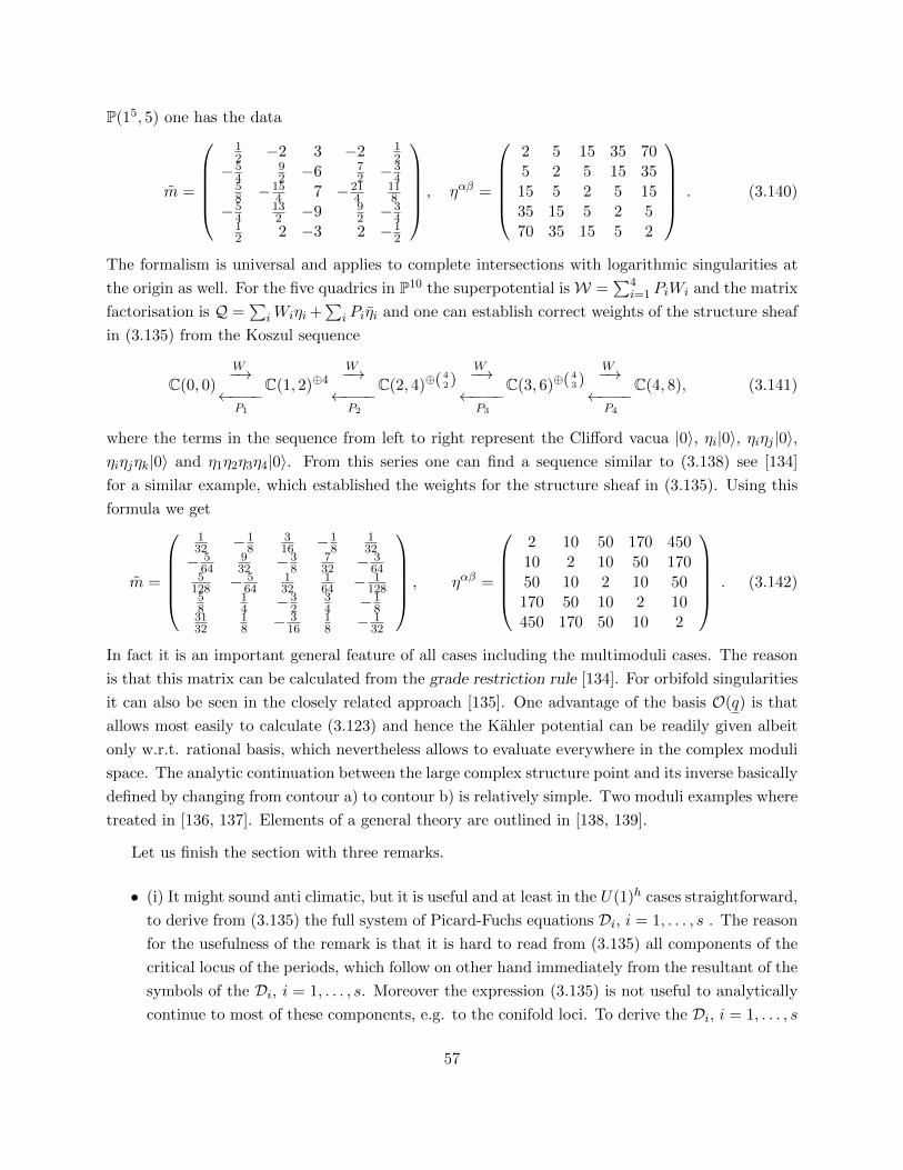
P(15, 5) one has the data
m =
12 −2 3 −2 1
2−5
492 −6 7
2 −34
58 −15
4 7 −214
118
−54
132 −9 9
2 −34
12 2 −3 2 −1
2
, ηαβ =
2 5 15 35 705 2 5 15 3515 5 2 5 1535 15 5 2 570 35 15 5 2
. (3.140)
The formalism is universal and applies to complete intersections with logarithmic singularities at
the origin as well. For the five quadrics in P10 the superpotential isW =∑4
i=1 PiWi and the matrix
factorisation is Q =∑
iWiηi +∑
i Piηi and one can establish correct weights of the structure sheaf
in (3.135) from the Koszul sequence
C(0, 0)W−→←−−−−
P1
C(1, 2)⊕4W−→←−−−−
P2
C(2, 4)⊕( 42)
W−→←−−−−
P3
C(3, 6)⊕( 43)
W−→←−−−−
P4
C(4, 8), (3.141)
where the terms in the sequence from left to right represent the Clifford vacua |0〉, ηi|0〉, ηiηj |0〉,ηiηjηk|0〉 and η1η2η3η4|0〉. From this series one can find a sequence similar to (3.138) see [134]
for a similar example, which established the weights for the structure sheaf in (3.135). Using this
formula we get
m =
132 −1
8316 −1
8132
− 564
932 −3
8732 − 3
645
128 − 564
132
164 − 1
12858
14 −3
234 −1
83132
18 − 3
1618 − 1
32
, ηαβ =
2 10 50 170 45010 2 10 50 17050 10 2 10 50170 50 10 2 10450 170 50 10 2
. (3.142)
In fact it is an important general feature of all cases including the multimoduli cases. The reason
is that this matrix can be calculated from the grade restriction rule [134]. For orbifold singularities
it can also be seen in the closely related approach [135]. One advantage of the basis O(q) is that
allows most easily to calculate (3.123) and hence the Kahler potential can be readily given albeit
only w.r.t. rational basis, which nevertheless allows to evaluate everywhere in the complex moduli
space. The analytic continuation between the large complex structure point and its inverse basically
defined by changing from contour a) to contour b) is relatively simple. Two moduli examples where
treated in [136, 137]. Elements of a general theory are outlined in [138, 139].
Let us finish the section with three remarks.
• (i) It might sound anti climatic, but it is useful and at least in the U(1)h cases straightforward,
to derive from (3.135) the full system of Picard-Fuchs equations Di, i = 1, . . . , s . The reason
for the usefulness of the remark is that it is hard to read from (3.135) all components of the
critical locus of the periods, which follow on other hand immediately from the resultant of the
symbols of the Di, i = 1, . . . , s. Moreover the expression (3.135) is not useful to analytically
continue to most of these components, e.g. to the conifold loci. To derive the Di, i = 1, . . . , s
57

that generate the ideal IPF , see section 3.7, we follow the observation made in [83] that the
classical intersection ring R(ξ) = ci1,...,inξi1 · · · ξin at a large radius point in coordinates47 at
zα = e−tα is given by
R(ξ) = C[ξ1, . . . , ξh]/Id(Si(ξ), i = 1, . . . , s), (3.143)
where Si is obtained as Si = limtα→∞Di(∂tα = ξα) and Id denotes the multiplicative ideal and
the ξ are the symbols of the differential ideal IPF . Consider now the monomials Di1 ·Di|I∗|
representing the Stanley Reisner ideal for a given triangulation. Pick a basis Ki of the Chow
ring and express the Di1 · Di|I∗| in terms of the Kj , j = 1, . . . , h. This yields polynomials
Si(Ki = ξi), i = 1, . . . , s − δ which generate part of the ideal Id. The full ideal can be
obtained by completing the Si(Ki = ξi), i = 1, . . . , s − δ minimally so that (3.143) holds.
Now we can act with the Sj(ξi = ∂ti), j = 1, . . . , s on any period say the one corresponding to
the structure sheaf Z(OW ). This brings down si monomials in the integrand, whose exponents
can be lowered by the relations xΓ(x) = Γ(x + 1), Γ(x)Γ(1 − x) = πsin(πx) and a redefinition
of the integration variables. This yields a relation between maximal order derivatives and
lower order derivatives of Z(O)W with polynomial coefficients in the e2πitα and constitutes a
linear differential operator annihilating all Z(O)W (q1, . . . , qh), i.e. a Picard-Fuchs operator
Di. The differential ideal of the latter completely determines these periods, if (3.143) holds.
The latter point should also hold in the case of non-abelian gauged linear σ-models, which
leads not to differential systems of generalized hypergeometric type, but rather to the Apery
type 48. The α(s) factor in (3.133) makes it slightly more non-trivial to lower the powers and
rewrite the integral in the standard form described above.
• (ii) We can study the period system on local Calabi-Yau spaces, by replacing the sections
W∆l= 0 of D0,l by the total space of the bundles ⊕rl=1O(−D0,l) over P∆∗ . This is the
obvious generalization of taking instead of the elliptic curve (quintic hypersurface) defined
as a section of the canonical bundle K in P2 (P4) the noncompact Calabi-Yau 3(5)-manifold
defined as the total space of the anti-canonical line bundle O(−3)→ P2 (O(−5)→ P4). This
is implemented by the following change in the integrand of (3.135)
sinh(πl(α)0j sα)→
sinh(πl(α)0j sα)
sα. (3.144)
This process can be done successively leading to an increasing number of non-compact direc-
tions.
47Note that in this section tα denotes not the quantum corrected Kahlerparameter, which is defined in 3.88.48Only the one moduli cases of Apery type, like the Grassmannians for which higher genus invariants have been
calculated in [140], have conifold loci in different distance from the large complex structure point limt→∞. This is anecessary condition for fast enough convergence of the analytic continuation from the conifold to the large complexstructure point, that would be needed to prove the irrationality of ζ(2m+1) occurring in the periods of CY 2m+1-foldsfor m > 1 at infinity due to (3.120) in (3.124). We thank Sergei Galkin to point this fact out.
58

• (iii) Finally we like to point out that by applying a Legendre transform to the etα variables
in the integrals (3.135) one gets periods governing the I-functions of the A−model on P∆∗ .
This can be done partially on some of the etα . In this case one gets more involved del Pezzo
manifolds W given by constraints that render c1(W ) > 0. In this case one gets instead of
hypergeometric or Apery-like functions Bessel like functions that have different asymptotic
expansion. The transitions matrices m, m and n can be related to the Stokes matrices of
that system.
3.11 Minimizing the flux superpotential
The superpotential in type IIB and F-theory can be expanded in terms of a basis of periods as
W =
∫Mn
Ωn(z) ∧Gn =∑α
nαΠα(z) , (3.145)
where
Πα(z) =
∫Γα
Ωn(z), Γα ∈ Hprimn (Mn) . (3.146)
In the presence of space filling branes internally wrapped on special Lagrangian branes L, Γα can
be more generally viewed as a chain integral in relative homology Hreln (M,L) ending on L and con-
tributing likewise to the space-time superpotential. The superpotential W transforms in L and the
covariant derivative Di = ∂i+∂iK enters the minimization conditions for the superpotential spelled
out for type IIB vacua in [31]. If one denotes by ai the chiral N = 1 superfields the corresponding
parts of the effective action can be expressed in terms of a generalized Kahler function 49
G(a, a) = K(a, a) + log |W (a)|2, (3.147)
which determines the scalar potential as
V = eG(GiGG
i − 3). (3.148)
Note that in general the ai are not only the complex moduli, but all moduli of the effective theory,
i.e. also the Kahler moduli and the dilaton. These can be treated separately as long as they
contribute at least approximately additively to G. I.e. if K = Kcs+Kks+Kd and W = WcsWksWd,
which assumes decoupling properties. In particular as far as the dilaton is concerned this is a weak
coupling approximation50. In this case the contribution of the complex moduli a is
Vcs = eKcsGaa|DaW |2 . (3.149)
The mass of the N = 1 gravitino is given by
m3/2 = exp(G) = exp(K/2)|W | . (3.150)
49That transforms with G(a, a)→ G(a, a) + f(a) + f(a) under gauge transformations Ω→ Ωef(a).50It is only in this section that we distinguish between K (W ) and Kcs (Wcs) in the other sections K (W ) simply
mean Kcs (Wcs).
59

Generically minimisation of V , i.e. ddaiV = 0 leads to anti de Sitter space at V (amin). To find a
N = 1 supersymmetric vacuum one needs all auxiliary fields to vanish
H ı = Gıj |W |eK2 (∂jK +
1
W∂jW ) = 0 . (3.151)
Since these terms are all positive they have to vanish individually. In particular if GıjeK2 as well
as ∂jK are generic at the minima this means
W |min = 0, ∂iW |min = 0 (3.152)
is a supersymmetric vacuum. More generally one searches for
DiW = 0 . (3.153)
If the vacuum manifolds represent smooth Calabi-Yau fourfolds one has therefore the following
conditions at the minima of the superpotential [24], see also [141].
• M1) For the superpotential (2.1) Wcs(a) = 12π
∫M4
Ω(a) ∧ G4, the first condition in (3.152)
means by (3.10) that G4 cannot be of type (0, 4). The second equation and (3.44) and Griffiths
transversality (3.43) tells that it cannot be of type51 (3, 1) and since W is holomorphic G4
has to be of type (2, 2).
• M2) For the superpotential (2.2) Wks = 14π
∫M4
J2(t) ∧ G4 the second condition in 3.152
implies that J ∧G4 = 0, i.e. that G4 is primitive. It follows then by M1.) and (3.9) that G4
is selfdual. The first condition in (3.152) imposes no further constraint on Wks.
It is hence possible to restrict many complex moduli by turning on a primitive flux G4 on
an algebraic (2, 2) cycle [G4] as long as the minimum configuration is smooth. Like for K3 the
existence of an algebraic cycle restricts the complex family of Calabi-Yau fourfolds to the analog of
the Noether-Lefshetz locus 52. It can be argued from deformation theory that a single (2, 2) class
could in principle restrict all complex moduli. In practice one try to find restricted but smooth
configuration of the algebraic constraints, which allow the algebraic cycle to exist. E.g. one can
insist that there is an algebraic P2 in the sixtic in P5 by restricting the general constraint to the
form
W ∆
= x1f(1)5 (x) + x2f
(2)5 (x) + x3f
(3)5 (x) = 0 , (3.154)
where the f(i)5 are arbitrary homogeneous polynomials of degree 5. For this constraint the P2
specified by x1 = x2 = x3 = 0 is always on the sixtic and some complex structure deformations
51If one imposes just DiWcs = 0 one can, as DiΩ spans H3,1 by the T.-T. Lemma, only conclude that G4 is not oftype (3, 1) and (1, 3). Still G4 will be selfdual as (4, 0) and (0, 4) are selfdual.
52We would like to thank Sheldon Katz for pointing out many examples of this kind, including a preliminaryanalysis that by this method one can restrict the sixtic to the parameter family that we analyze in section 3.9.3. Wealso were not aware of the following deformation argument.
60
are absent. Setting up the same calculation we used at the end of section 3.9.3 to find the number
of lines on the sixtic one finds that the rank of the quotient bundle S6QP2 describing P2 that lie
on the sixtic is 28, while the dimension of Gr(3, 6) is 9. Hence the algebraic cycle obstructs 19
complex structure moduli. This can be also counted by counting the polynomial defomations of
W ∆
modulo automorphisms.
This method is closely related to the one discussed in (3.6) and 3.11.3). In particular these
configurations are also at fixpoint of the induced automorphisms discussed in (3.6). In F-theory
the approach gives a simple characterization of the allowed fluxes. These are those primitive
algebraic cycles, which preserve the Weierstrass forms. In order to study the actual scalar potential
at the fixed loci in Mcs, to find the flux quanta relative to an integral basis or to find the Kahler
potential one has to determine the integral basis at the degeneration locus.
Note that in N = 2 backgrounds the conditions (3.152) are equivalent to the conditions for an
attractor point for a supersymmetric black hole of mass
M2BPS = eKcs |W (a)|2, (3.155)
where the gravitino mass is identified with the Bekenstein-Hawking entropy of the black hole at
the attractor point [31]
S = πe−KHm23/2 . (3.156)
Here H are the hypermultiplets, i.e. the dilaton plus Kahler moduli in type IIB compactifications.
This correspondence allows to use some results on attractors in the next sections.
Now suppose that there is a symmetry Γ : Mcs → Mcs acting on the complex moduli space
and H ı are generic enough equivariant Morse functions w.r.t. Γ, then by the standard argument H ı
vanish only at the fix-point locus fΓ of Γ. However the local Torelli theorem holds for Calabi-Yau
manifolds and assures that one can pick certain Πi(z), i = 1, . . . , hn,1 to be faithful local coordinates
near fΓ so that one can always pick nα in W to H ı generic enough Morse functions.
3.11.1 Arithmetic of orbifolds and supersymmetric vacua
We have seen in section (3.6.1) that finite order discrete symmetries that act subject to the condi-
tions G1) and G2) on Mn have an induced action on the single cover description of Mcs.
The first observation is that by turning on fluxes on the invariant periodsW = |G|
∑i niΠ
diag i0
under G the theory is driven to the sublocus S in the moduli space. Here we multiplied by the
order |G| of the group G and pick ni ∈ Z, which guarantees that the flux is integral. Let us denote
as before the invariant moduliai and the non-invariant moduli ai. Then (3.33) is the model for the
local behavior of the periods near an orbifold point ai = 0 written in terms the local vanishing non
invariant modulus a. Hence by (3.33) we can conclude that
∂aiW (ai,
ai) = 0 . (3.157)
61

Because of the positivity of the individual terms in (3.151) e.q. (3.157) is a necessary condition to
have a supersymmetric vacuum and drives the theory to the invariant subspace S [31]. Moreover at
an orbifold point the Kahler metric is regular as W inv∆ = 0 is transversal. Now if the flux conditions
∂ai
W (ai,
ai) =
W (ai,
ai) = 0 drive the flux to the supersymmetric locus W (ai,
ai) = 0, then all
conditions for the supersymmetric vacuum are met.
If k > 2 then we can also put the flux on W =∑
i ciΠdiag ik>1 and get
∂aiW (ai,ai)S = W (ai,
ai)S = 0 . (3.158)
Again since at the orbifold point the Kahler metric is regular this solves the supersymmetry con-
dition already on the entire subspace S. Of course the question here is whether one can pick the ci
so that W =∑
i ciΠdiag ik>1 is an integral flux potential. If there is just one prime orbit in G of order
p without homological relations among the cycles Γi this is impossible, because of the roots of p in
the coefficients ci as explained in section 3.6.1. In this case one can approximate the roots of p to
arbitrary precision by a rational number. The corresponding large denominators can be cancelled
by choosing a large common factor in the integer flux quanta. This can lead to hierarchically small
breaking of supersymmetry.
Let us describe simple situations in which the theory can be driven to an orbifold point through
integral fluxes. Based on the results of [71, 72] the orbifold point a0 = 0 of the degree six hypersur-
face∑4
i=1 x6i +2x3
5−6a0∏5i=1 xi=0 in P(1, 1, 1, 1, 2)/(Gmax
ph = Z26 × Z2) was found to be an attractor
point in [32]53. The latter can be viewed as the mirror of the degree six hypersurface in P(1, 1, 1, 1, 2).
The model has an additional Z6 symmetry x4 → x4α, a0 → a0α−1 with α = exp(2πi/6). This
fulfills G1) in section 3.6.1, but not G2). Hence there will not be a resolvable Calabi-Yau orbifold
M3/Z6. The rotation of a0, the coefficient of the inner point ν0 cff. (3.18), is a special case for
two reasons 54. Firstly even though G2) is violated Ω is invariant because of (3.51). Secondly the
invariant subspace in the moduli space cannot be the moduli space of another Calabi-Yau manifold,
as eliminating the inner point leaves the class of reflexive polyhedra. It follows in particular that Γ0
must be trivial in homology so that there will be no invariant period. From these facts and the ones
stated in section (3.6.1) it follows that solutions near a0 = 0 take the form Πp =∑∞
n=1 cn(a0αp)n 55.
One can pick a basis Πorb = ($2, $1, $0, $5)T and using the Mellin-Barnes integral continuation
one finds [72]
Πlcs =
0 0 −1 0−1
3 −13
13
13
0 −1 1 01 0 −3 −2
$2
$1
$0
$5
. (3.159)
53There are four families of hypersurfaces of degree k = 5, 6, 8, 10 in weighted projective space P4(w) [71, 72] andmany formulas can be written in terms of k and wi, i = 1, . . . , 5.
54For the cases discussed in [67] it is also a point with an exactly solvable rational super-conformal field theorycalled the Gepner model.
55The cn = −i 23π4
k|Gmaxph|
γnei πk
(k−1)n
sin(πnk )Γ(n)∏5i=1 Γ(1−nwi
k )with γ = k
∏5i=1 w
−wi/ki are calculated as the solutions to the
PF-equation at this point. |Gmaxph | = 3322 for the k = 6 case.
62

So we learn that W = k(F1− 3X0) +nF0 +mX1 ∼ a0(3k−m−n) +O(a20) with (3k−m−n) = 0
and k,m, n ∈ Z subject to this condition generates a two parameter lattice of flux superpotentials
which drives the theory to the orbifold point σ = $1$0∼ a0 = 0 where one has W = 0 and
∂σW = 0 at σ = 0 hence a minimum that is equivalent to an attractor point of an N = 2 black
hole with electric and magnetic charges. Here we introduced the flat orbifold coordinate σ56 . The
reason behind that solution is of course just the arithmetic relation α5 = −α2 = α0 − α1 of sixth
order roots. For k = 5 there is no arithmetic relation between the fifth roots and for the k = 8
and k = 10 cases the arithmetic relations between the roots that would lead to integral fluxes
correspond to cohomologically trivial fluxes. Note that in these special cases with no invariant
period eKcs ∼ 1/|σ|2 has a singularity at σ = 0, so that the contribution of the complex structure
moduli to V (3.149) is positive despite the fact that ∂σW ∼ σ and KσW ∼ σ vanish at σ = 0 [31].
For the general orbifold one has a non-vanishing invariant period. This implies that eKcs is regular
at S = 0 and one gets a supersymmetric vacuum manifold.
For the degree six Calabi-Yau fourfold X6(16) in P5 we can use (3.113) to establish a flux
potential W (k,m, n) that behaves like
W = 12(m+n)X0+2(5k+3m+n)X1+(7k+5m+3n)H+4(6m+5n−2k)F1−12kF0 ∼ a20+O(a3
0) ,
(3.160)
for k, n,m ∈ Z arbitrary. Using the solutions(3.9.3) one concludes that within this three parameter
family of flux potentials there is a one parameter family
W (0,m,m) ∼ a30 +O(a4
0) . (3.161)
The explicit expression for the integer basis of periods and the Kahler potential shows with σ =$1$0∼ a0 that DσW ∼ σ2, while the asymptotic behavior of Gaa is regular Ga0,a0 =
Γ6( 56)Γ6( 1
3)Γ6( 1
6)Γ6( 23)
and
eKcs ∼ 1/|σ|2. Therefore the scalar potential
V = eKcsGσσ|DσW |2 ∼ |σ|2 , (3.162)
vanishes at the orbifold point σ = 0. It is quite significant that we can first reduce the dimension
of the moduli space of the sextic to a one dimensional monodromy invariant subspace S by the
Z46 maximal phase symmetry or eventually by finding appropriate algebraic (2, 2) and fix the last
modulus at the Z6 orbifold or Gepner point with vanishing scalar potential. With a different choice
of m,n, k one can add a positive constant to V . Because of the general rationality of the transition
matrix m due to the grade restriction rule cff. (3.142), this result generalizes immediately to other
Fermat hypersurface in weighted projective spaces Xd(w1, . . . , w6), i.e. with wi|d, because the
latter condition together with the Calabi-Yau condition∑
iwi = d implies that d ∈ 2Z, which
makes the cancellation of non-trivial roots possible. Since among the Fermat hypersurfaces one has
hundreds of elliptic fibrations the mechanism is relevant for F-theory, with the additional bonus
56See [142] how to chose flat closed and open orbifold coordinates.
63

that the discrete orbifold symmetries have the potential to create selection rules that might lead to
approximate hierarchies among the Yukawa couplings.
Let us conclude the section with the general criterium to have an integral superpotential on the
non-invariant cycles: If the finite group Gfix that fixes S has arithmetic relations among its roots
that do not correspond to cohomological relations between the cycles in its orbit it is possible to
find an integral flux superpotential W that has S as its supersymmetric moduli manifold.
3.11.2 The nodal points and supersymmetric vacua
Let us discuss now the behavior of the superpotential at the most generic local singularities
n+1∑i=1
ζ2i = ε2 = δc , (3.163)
of a n dimensional complex manifold, i.e. when a cycle ν with the topology of a sphere Sn, which
is the real section of (3.163), shrinks to zero size. The singularity is called a node and the codim
one sublocus δc = 0 in the complex moduli space is called the conifold divisor. The integral over
the cycle ν can be calculated iteratively in ε as was done for n = 3 in [99, 71, 72]. To give a
dimensional argument for its leading behavior in ε for various n, it is convenient to integrate over
γ in (3.47). One can do this in a patch of the toric variety where the local form of Ω becomes
Ω = a0dx1∧...∧dxn∂xn+1W∆(x,a) . Moreover one always finds a coordinate transformation xi → ci +
∑n+1k=1 c
ki ζk
so that locally W∆(x, a) = −ε2 +∑n+1
i=1 ζ2i + O(3) and η = ∂xn+1W∆(x, a) =
∑n+1i=1 diζi + O(2),
where ζ, η and ε have the dimension of a length which sets the order parameter. It follows from
the dimension of Ω = a0Jac(∂x∂ηi
)dη1∧...∧dηn
η that to leading order 57∫Sn
Ω ∼ εn−1 = (δc)n−1
2 . (3.164)
This behavior at the conifold divisor can be readily checked for the mirrors of degree k hypersurfaces
in Pk−1, where the PF-differential operator is derived from the GGKZ method to be
Dk = θk−1 + (−1)k−1kzk−1∏i=1
(kθ + i), (3.165)
where θ = z ddz and z = 1
kkak0and δc = (1 + (−1)k−1kkz), by calculating the indicial equations for
the solutions near ∆c(a0) = 0. Examples of shrinking S4’s in more general fourfolds are discussed
in section 3.9.3.
One of the most famous predictions of N = 2 Seiberg-Witten theory is the existence of massless
BPS monopoles [143]. The corresponding one loop β-function for the gauge coupling, as encoded
57The proportionality constant is easily calculated by making a further orthogonal transformation on ζi → ηi sothat η becomes one of the coordinate axes. Then one can introduce spherical coordinates and perform the integral.This can be turned into an iterative scheme, but it is easier to get the subleading terms from the PF equation.
64

in the derivative of FΓ w.r.t. Xν , generates a shift monodromy like in (3.100). Eq. (3.164) does
not allow vanishing periods on elliptic curves n = 1 for the canonical (1, 0) form. The conclusion
is avoided in Seiberg-Witten by using a meromorphic one form λ, which descends from the (3, 0)
form of a Calabi-Yau 3-fold in the local limit. In this case (3.164,3.155,3.100) allows massless BPS
states as well as logarithmic shifts. One may see this as a dimensional argument that these gauge
theory effects find their natural explanation in string theory.
According to the Lefschetz formula with some sign corrections by Lamotke [144], an n-cycle Γ
transforms along a path in the moduli space encircling the conifold divisor ε = 0, where the Sn =: ν
vanishes, with positive orientation with the monodromy action on Γ that is either a symplectic -
for n- odd or an euclidean reflection w for n-even, i.e.
w(Γ) = Γ + (−1)(n+2)(n+1)/2〈Γ, ν〉ν . (3.166)
The self intersection of the sphere itself is given by
〈ν, ν〉 =
0 , n odd
(−1)n/2 · 2 , n even .(3.167)
Let us now discuss the two cases in turn:
• n odd: Due to the non-degenerate symplectic pairing the vanishing cycle ν intersects a dual
cycle Γ and in order to realize (3.166) the periods over these cycles degenerate in the local
parametrization δc = 0 for n odd like
Xν =
∫ν
Ω = δn−1
2c
∞∑k=1
ck(a)δnc ,
FΓ =
∫Γ
Ω =(−1)(n+2)(n+1)/2
2πiXν log(Xν) +
∞∑k=0
bk(a)δkc .
(3.168)
Usually one cannot determine the integral and cycles directly and rather solves the Picard-
Fuchs equations near ε = 0, but the Lefschetz formula fixes the relative normalization of the
solutions so that T =
(1 01 1
)is the unipotent monodromy when for a path that encircles
δc = 0 counter clockwise.
It has been argued [145],[31] that putting a flux on the S3 in M3, i.e. the non-invariant
periods drives the theory towards the conifold58.
• n even: The Sn intersects with itself and so the typical local behaviour for the K3, 4-folds
etc is w(ν) = −ν, for a single Sn and hence
Xν = δn−1
2c
∞∑k=1
dk(a)δkc , (3.169)
58Note that in general at the conifold locus of compact examples one has several Sn with topological relationsvanishing, which in the transition are blown to P1 with relations. This fits perfectly the N = 2 Higgs mechanismwith abelian gauge groups [146]. More complicated situations with non-abelian gauge symmetry enhancements arediscussed in [76],[75].
65

e.g. for 4-folds one finds Xν = δ32c etc. This leads to a Z2 monodromy.
If we put a G4 flux on the S4, which is at least a rational cohomology cycle, then
W |δc=0 = 0, ∂δcW |δc=0 = 0 . (3.170)
More accurately in the right local coordinate Xν one has from the local limit of the Kahler
potential
DXνW = 0 . (3.171)
This means that we can always find a rational flux, which drives the theory towards the most
generic singularity of the 4-fold, where we find a supersymmetric vacuum.
3.11.3 Flux superpotential and sub-monodromy problem
In the section 3.7 we explained how to get the Picard-Fuchs or equivalently the Gauss-Manin
connection for W inv∆ (a, Y ) on the subspace S of the moduli space and argued that the latter defines
a sub-monodromy problem on the invariant periods. Here we want to investigate the properties of
the flux superpotential that can drive the complex moduli to the invariant subspace S.
Local considerations: Let us start with the local properties of the Gauss-Manin connection locally
near S. We introduce the following notations: ai, i = 1, . . . , hn−1,1(Mn) are gauged fixed complex
structure variables. We split them into variables along the invariant subspaceai,i = 1, . . . ,dim(S)
and the ones transversally to S ak, k = 1, . . . , codim(S) so that ak = 0 characterizes S. The
Frobenius algebra property FAnd.) is equivalent to the local Torelli and so we can introduce locally
periodsΠi along and Πk transversally to S and write Π(a) = (
Π(a), Π(a)). Using the pairing
between χik,n and Γi we write the Gauss-Manin connection (3.56)59 for the non-invariant variables
ai ∂ai +
Γa
ai,a
Γaai,a
Γaai,a
Γaai,a
( Π
Π
)= 0 , (3.172)
and the one for the invariant variables∂ai
+
Γaai,a
Γaai,a
Γaai,a
Γaai,a
( Π
Π
)= 0 , (3.173)
For ΓS to be a closed sub-monodromy problem the terms Γa
ai,a
= Γaai,a
= Γaai,a
= 0 have to vanish
at S.
59In fact this connection can be easily numerically integrated along paths around ∆i to obtain all monodromymatrices Mi as the precision even for multimoduli problems is good enough to approximate the integers in Mi. Wethank Duco von Straten for pointing this out to us.
66

• Let us now consider a flux on the non-invariant periods Π. From equation (3.172) and the
fact that Γaai,a|S = 0 one sees that ∂aiΠ has to vanish, when Γaai,a does not have a pole in
ai of order one or higher. This is not the case at orbifold divisors, irrespectively of the fact
whether the latter is abelian or non-abelian. Similar ∂ai
Π = 0, because Γaai,a|S = 0 and
Π stays generically regular as
Mn is transversal. Differently as in the somewhat particular
orbifolds discussed in (3.11.1) eKcs and ∂aiKcs have no pole generically at S, again becauseMn is transversal for generic values of
ai. Therefore if the superpotential is entirely put on
the Π periods DiW |S = 0 and also V |S = 0. In the case of the conifold singularities we
refer to [145],[31] and the result in section 3.11.2 to reach the same conclusion, namely that
putting the fluxes on the non-invariant periods drives the theory to the supersymmetric locus
S. One can also argue that the auxiliary fields (3.151) are equivariant Morse functions under
the actions defined in section (3.6.1) and (3.6.2) and therefore have to vanish at the fix point
set S of these actions.
• Next we consider a flux on the invariant periodsΠ. Again we conclude that ∂ai
Π|S = 0
and since eK is bilinear in the periods also ∂aiK|S = 0 hence DaiW |S = 0. Of course this
means only that we found a necessary condition to have a vacuum. In addition one has to
have DaiW = 0. Again one makes a simple localization argument [147], provided that one
has established a group action on the periods like in (3.36) and the invariance of K under it.
Then one can differentiateΠ(g ·a) =
Π(a) and K(g ·a) = K(a) with respect to ai to conclude
from g∂aiΠ(g · a) = ∂aiΠ(a) and g∂aiK(g · a) = ∂aiK(a) that ∂aiΠ(a) and ∂aiK(a) has to
vanish at the fix set g · a = a and so again that DaiW |S = 0. Such arguments are used also
in [148][149].
Global considerations: While ΓS is a subgroup of ΓM it should be made clear thatΠ is not an
invariant subspace under the action of ΓM. An illustrative example for this was given in [150],
where the periods of the pure N = 2 SU(2) Seiberg-Witten appear in a decompactification limit
of a global Calabi-Yau 3-fold defined as hypersurface X12(1, 1, 2, 2, 6) in the weighted projective
space P(1, 1, 2, 2, 6) . In this case the invariant periods transform under the ΓS = Γ0(4) ∈ SL(2,Z)
sub-monodromy group in the Seiberg-Witten limit within the compact Calabi-Yau 3-fold. Eq.
(5.4) shows that invariant and non-invariant periods mix under the full original monodromy group
ΓMcs with rational coefficients. Such a rational mixture should be generic, when a sub-monodromy
problem on the invariant periods can be defined in the sublocus S. It is therefore natural to
conjecture that the flux quanta on the non-invariant periods, that drive the theory towards S by a
flux superpotential W can always be chosen to be integral.
Based on the examples and the symmetry considerations we close the section with a conjecture
concerning the sublocus S and the sub-monodromy system described in section 3.7. Whenever
there is a sublocus S so that IPF |S describes a closed sub-monodromy system and S is not at
67

the boundary of Mcs where Mn degenerates, then S is at the fix point of a group action on Mcs
induced from discrete group action on Mn. Depending on the arithmetic there might be an integral
flux that drives the moduli to S. All other integral fluxes drive the moduli to a subloci S at the
boundary of Mcs.
4 Compact Calabi-Yau manifolds with no gauge group
We will construct families of toric hypersurface with elliptic fibrations of type D5, E6, E7 and
E8, which have no non-abelian gauge symmetry enhancements. The significance of these families
is that for a given base and fibre choice they have the most general complex structure. In this
sense they can be seen as clean sheets on which by suitable specializations of the complex structure
induced by G4 fluxes, singularities along divisors yield non-abelian gauge symmetry enhancement
and by further enhancement of the singularity in higher codimension the matter sectors and Yukawa
couplings might be imprinted. It is a general strategy to analyze these singularities by blowing them
up to a smooth variety, which is a valid approach in our case as well that we pursue in section 6.
However in F-theory one has to keep in mind that these blow ups which involve finite volumes
exceptional divisors in the fibre are unphysical. The actual breaking of the gauge symmetry is by
deforming the singularities i.e. by Higgsing, by flux breaking or by Wilson lines.
As explained in section 3.2 the anticanonical divisor has to be semipositive on any effective curve.
The simplest possible choice for the basis are 84 Fano basis B3 [58]. A much more wider class are
the almost toric basis P∆ corresponding to the 4319 3d reflexive polyhedra that are classified to
construct K3 as hypersurfaces [151]60.
The advantage of the construction is that there exists always triangulations of ∆5 compatible
with the fibration structure and that all classes of the base are torically realized as classes of the
fourfold M4.
We first will classify the Fano or almost Fano smooth projective toric varieties, which allow for
a P1 fibration over B2 and have therefore a dual heterotic description. Ultimately they will be all
contained in the list of 4319 P∆ mentioned above. It has nevertheless advantages to start with B2.
The reason is that, while F1.) is trivial to establish, to check for the compatible triangulations
required in F2.) for a given B3 takes time.61
There is no complete list of reflexive polyhedra in 5d and we are not trying to classify all possible
toric 3d basis as in [152], which lead to a Weierstrass with smoothable Kodaira fibers, only the ones
which are already smooth. The reason why this is almost as useful is that giving blow ups in the
base or any number of divisors on which to impose a gauge group leads to a sub-point configuration
60The 18 toric almost Fano B2 were classified, e.g. by Batyrev.61This applies similarly to the list of [152], which lists all possible toric basis which allow for a compact Weierstrass
model. It should be implicit in the complete list of 4d reflexive polyhedra but checking for F2.) given F1.) is difficult.
68

of points in ∆ or ∆∗ and there are programs like Palp, which can check whether these points can
be completed to a reflexive polyhedron.
4.1 Rational fibred basis over almost Fano varieties
For comparison with the heterotic string we construct bases Bn−1 that exhibit a P1 fibration
πr := P1 → Bn−2, which by the adiabatic extension of the heterotic type II duality is identified
with the base of the compactification manifold Zn−1 πh : Ehet → Bn−2.
The gauge and gravitational anomaly condition is the Donaldson-Uhlenbeck-Yau condition for
stable heterotic bundles
λ(V ) = λ(V1) + λ(V2) + [W ] = c2(TZn−1) , (4.1)
where the bundle V1 is the one of the first E8 and V2 of the second E8 and λ(V ) is in the fourth
real cohomology, e.g. the second Chern class λ(V ) = c2(V ) for SU(n), but for Spin(n) the first
Pontryagin class λ(V ) = p1(V ). Further to admit spinors one needs
c1(V1,2) = 0 mod 2 . (4.2)
For the case n = 3 this yields the 6d F-theory compactification dual to the heterotic string compact-
ified on an elliptically fibred K3 and the only option for the P1 fibration over B1 are the Hirzebruch
surfaces Fm. Since∫K3 c2(TK3) = 24, one denotes
t = 12− πh∗(λ(V1)) , (4.3)
and considers for symmetry reasons only 0 ≤ t ≤ 12.
It has been observed in [18] and proven in [23] that one can identify t with the twisting of
the fibre P1 in Ft. Moreover only for t = 0, 1, 2 the bundles V1 and V2 can be generic enough in
both E′8s to break the gauge group completely. The goal of the subsection is to find the analogous
geometric condition for hypersurfaces in toric ambient space of F-theories with heterotic duals in
4d. The data of πr are a projectivized bundle O(1)⊗ T , where T is a line bundle over Bn−2. Let
us denote α = c1(O(1)) on Bn−2 and t = c1(T ) and specialize to n = 4, i.e. compactifications to
4d. Then by adjunction c(B3) = (1 + c1(B2) + c2(B2))(1 + α)(1 + α + t) and using α(α + t) = 0
one can calculate by integrating over the P1 fibre the integral∫B3
c31 = 6
∫B2
c21 +
∫B2
t2 , (4.4)
in terms of integrals over the base B2. In the most general toric construction B2 is defined as one of
the sixteen toric almost Fano varieties B2 = P∆(i) , i = 1, . . . , 16 classified by Batyrev and displayed
in figure 1. We like to know which line bundle T leads to F-theory without gauge groups.62
62By Hirzebruch-Riemann Roch index theorem all rational 3 folds have∫B3c1c2 = 24, hence (4.4) is the only
variable contribution to the Euler number (4.18).
69

1
12/72:4(2)
9/27:2(0)
1
12/72:4(2)
9/27:2(0)
2
8/24:3(0)
10/48:4(1)
2
8/24:3(0)
10/48:4(1)
6/18:5(0) 6/24:6(1)
8/36:5(1)
10/48:4(0)
18/144:3(0) 12/27:4(0)
6/18:5(0) 6/24:6(1)
8/36:5(1)
10/48:4(0)
18/144:3(0) 12/27:4(0)
887
6/18:5(0)
8/36:5(0)
7
6/18:5(0)
8/36:5(0)
10
6/18:5(0)
6/24:6(2)
12/60:3(0)
18/144:3(0)
30/360/2(0)
6/24:4(0)
12
5/15:6(0) 6/24:6(0)
8/36:5(0)6/72:4(0) 8/36:5(0)
12
5/15:6(0) 6/24:6(0)
8/36:5(0)6/72:4(0) 8/36:5(0)
116/24:6(0)6/24:6(1)
12/72:4(0)
10/48:4(0)
12/72:4(0)
18/144:3(0)
8/36:5(0)
5/15:6(0)
9
6/18:5(0)
6/24:6(1)
10/48:4(0)12/72:4(0)
8/36:5(0)
13
412:7(0)
6/24:6(0)
18/144:3(0)
12/72:4(0)
12/48:4(0)
12/72:4(0)
6/24:6(1)
13
412:7(0)
6/24:6(0)
18/144:3(0)
12/72:4(0)
12/48:4(0)
12/72:4(0)
6/24:6(1)
14
4/12:7(0)6/24:6(0)
6/24:6(0)
12/72:4(0)
8/36:5(0)
8/36:5(0)
12/72:4(0) 6/24:6(0) 6/24:6(0)
14
4/12:7(0)6/24:6(0)
6/24:6(0)
12/72:4(0)
8/36:5(0)
8/36:5(0)
12/72:4(0) 6/24:6(0) 6/24:6(0)
16
3/9:8(0)6/24:6(0)
12/72:4(0)
16
3/9:8(0)6/24:6(0)
12/72:4(0)
15
4/12:7(0) 6/24:6(0)
8/36:5(0)
12/72:4(1)
z
y
x
z
x
y y
x
z
y
x
z
z
y
z
x
y
F
F
G
4
8/24:3(0)
4
8/24:3(0) 6/24:6(3)14/72:2(0)
5
7/21:4(0)
10/48:4(0)
8/36:/5(1)
5
7/21:4(0)
10/48:4(0)
8/36:/5(1)
18/144:3(1)
x
66
12/60:3(0)6/24:6(2)
18/144:3(0)
12/72:4(1)
7/21:4(0)
12/72:4(0)
3
8/24:3(0)
8/36:5(2)
12/60:3(0)
3
8/24:3(0)
8/36:5(2)
12/72:4(1)
12/60:3(0)
12/72:4(1)
F 12/72:4(0)
Figure 1: The 16 reflexive polyhedra ∆2 in two dimensions. When we refer to thepoints we denote the origin as ν0 the one to the right (for 13 right down) of the originas ν1 and numerate the rest counter-clockwise. The polyhedra are relevant for twoconsiderations in this paper: Firstly they are the toric basis for the F-theory basis∆B∗
3 : P1 → (B2 = ∆2) for those clean sheet models that have heterotic duals in theclassification in table 4.1. Secondly they classify toric elliptic fibres ∆∗F2 = ∆2 in (3.17).In this application one can read from the labels on the inequivalent points the Eulernumber and the number of Kahler classes according to formula (4.19) for 3-folds and4-folds.
70

The simplest example B2 = P2 [1] is given torically as P∆∗BFm= Fm defined by the complex hull
of the points u1 = (1, 0, 0), u2 = (0, 1, 0), u3 = (−1,−1,−m), w1 = (0, 0, 1), w2 = (0, 0,−1). It
has χ(Fm) = 6. The first Chern class of the bundle T specified by ∆∗B integrates to∫B2t2 = m2.
Here m is an example of a twisting datum and without restriction we can chose m ≥ 0. Let us
denote the divisors associated to the points νi by Dνi . Between toric divisors one has the relations∑i νi,kDνi = 0 for k = 1, 2, 3, e.g. it follows Du1 = Du2 = Du3 = F . The canonical class is
K =∑
iDνi = (3 +m)F + 2S, where S = Dw2 , a section of the fiber P1, and F are a basis of the
Picard group. The Mori vectors representing dual curves can be found at the circuits of the unique
star triangulation of ∆∗B [51] and are in this case (1, 1, 1, 0,−m;m − 3) and (0, 0, 0, 1, 1;−2). In
particular there is a curve h = SF , the hyperplane in the base P2, and the evaluation of K on h
is Kh = 3 −m. Hence ampleness of K yields the bound m < 3 and semi positivity m ≤ 3 and
precisely for these values ∆∗B is reflexive. Evaluating the contribution to c2(M4) from the base in
table 4.2, we find e.g. for the E8 fibre
11c21 + c2 = (11m2 + 69m+ 102)F 2 + 138FS . (4.5)
We can conclude that c2(M4) is even in terms of an integral basis of algebraic four-cycles for all m.
This is true as long as the coefficient of c21 in c2(M4) is odd, otherwise m has to be odd.
For the general case let ν(i)j , j = 1, . . . |∆(i)
2 \ ν0| = r be the points of ∆(i)2 defining the one
dimensional cones, then a P1 fibration over P∆
(i)2
is defined by the polyhedron ∆(i,m)3 , which is the
complex hull of the pointsu1 = (ν
(i)1 ,−m1)
......
ur = (ν(i)r ,−mr)
w1 = (0, 0, 1)w2 = (0, 0, −1)
, (4.6)
where mi ∈ Z are the twisting data, which have to be small enough for P∆
(i,m)3
to be (almost) Fano.
Of course in view of the relations between the divisors in the base only r − 2 twisting data are
relevant.
Let us discus the cases with two divisors in the base as examples. For B2 = F0 = P1 ×P1 the situation is a straightforward generalization of the above. Since Dν1 = Dν3 = F1 and
Dν2 = Dν4 = F2 one needs only say m3 and m4 and the Picard group is generated by F1, F2 and
S = Dw2 . The canonical class is K = (2 + m3)F1 + (2 + m4)F2 + 2S and the Mori vectors are
(1, 0, 1, 0, 0,−m3;m3−2), (0, 1, 0, 1, 0,−m4;m4−2) and (0, 0, 0, 0, 1, 1;−2). The strongest restriction
on positivity of K comes for the curves h1 = SF1 and h2 = SF2 namely m3 ≤ 2 and m4 ≤ 2, which
corresponds to entry 2 of table 4.1. Again we calculate the contribution to c2(M4) from the base
in table 4.2 for the E8 fibre type
11c21 + c2 = 2(11m3m4 + 23(m3 +m4) + 46)F1F2 + 92S(F1 + F2) , (4.7)
and get an even expression.
71

The Fano basis F1 is somewhat more interesting. We can pick the fibre of F1, Dν2 = Dν4 = F
and a section T = Dν3 of the fibre of F1 and the section S = Dw2 and get from h1 = ST and
h2 = SF constraints m3 ≤ 2 and m4 ≤ 3. However the case m3 = 2 and m4 = 0 is not admissible
as this polyhedron does not admit a Kahler star triangulation fulfilling F2.) of section (3.4.2). The
only one that exist is 3, 4, 6, 1, 2, 6, 2, 3, 6, 1, 4, 6, 1, 4, 5, 1, 2, 5, 2, 3, 4, 2, 4, 5 and
the offensive tetrahedron is63 2, 3, 4 as it involves three points in the base at different heights.
In fact it has volume two and the associated toric variety is therefore singular. It is interesting to
note that the anti canonical hypersurface M4 in P∆∗5with ∆∗5 build in (3.17) avoids that singularity
and has the Hodge data 64 2464(2)0 M14856
4(0) . I.e. from h11(M4) = 4 = h11(B3) + 1 we learn that the
fibration has no further singularities. However from (14856 − 12 × 24)/(12 × 60) = 60715 we see by
comparison with (4.18), which holds if M4 has only I1 fibres that M4 must have other non-singular
fibre types. For the almost Fano basis F2 we get form the semi positivity of K, m3 ≤ 2, m4 ≤ 2m3.
We find the following necessary conditions for the smoothness of M4∫B2
t2 ≤∫B2
c21 . (4.8)
However non-singularity and the existence of a triangulation respecting the fibre structure further
restrict the values to the ones listed in table 4.1.
Notice that in this construction the polyhedra of the base B2 represent all possible del Pezzo
surfaces albeit the members of the series dnP2, i.e. 0 ≤ n ≤ 8 blow ups of P2, are for n > 3 realized
at special values of their moduli. In particular the reflexive polyhedra 15, 16, 13, 10 in figure 1 are
specializations of the D5, E6, E7, E8 del Pezzo’s. The smooth elliptic fibred CY 4-fold will have
h11(M4) = h11(B2) + 2 + s, where s is the number of sections of the elliptic fibre.
One might ask whether one can also realize the half K3 or d9P2 as heterotic basis. Then c31 = 0
and one expects from (4.18) that χ = 288 independent of the fibre type. This is not describable as
a toric base, e.g. because of formula (4.10), but it can be realized as an r = 2 and s = 0 complete
intersection in (3.17). An interesting case was constructed in [4] as a complete intersection of two
polynomials in P2 × P1 × P1 × P2 of degree (3, 1, 0, 0) and (0, 1, 2, 3) respectively. This corresponds
to the E6 fibre type. In the language of section (3.4.1) we get ∆∗ as the convex hull of the points
which describe the Pk factors, each given by a simplex with vertices, e(l)1 , . . . , e
(l)k ,−e
(l)1 − . . .− e
(l)k .
We consecutively label the vertices with the indices 1, . . . , 10. The nef-partition is given by D0,1 =
D1 + D2 + D3 + D4 and D0,2 = D5 + D6 + D7 + D8 + D9 + D10 and the Euler number is indeed
χ = 288, while h11 = 12, h3,1 = 56 and h21 = 28. A remarkable property in these models is
that they allow an infinite number of rigid divisors, which all contribute to a non-perturbative
superpotential [4]. The existence of the divisors can be seen by lifting rational curves in the del
63In a star triangulation all tetrahedra contain the origin which is therefore not indicated.64We give the complete Hodge data in the form
h31(t31)h21
Mχh11(t11), where t11 means twisted contributions from points
in dual one and three faces, which indicate non rational divisors Poincare dual to the corresponding (1, 1) forms andvice versa for h11(W4) = h31(M4).
72
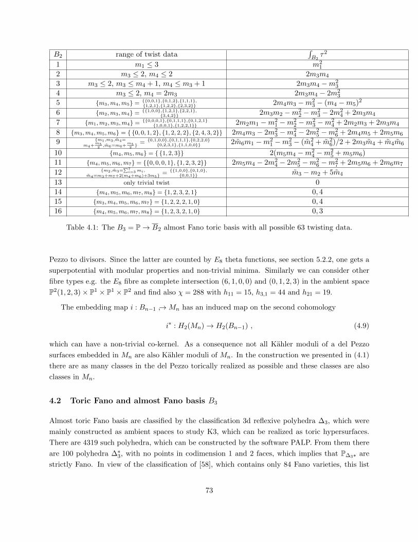
B2 range of twist data∫B2τ2
1 m1 ≤ 3 m21
2 m3 ≤ 2, m4 ≤ 2 2m3m4
3 m3 ≤ 2, m3 ≤ m4 + 1, m4 ≤ m3 + 1 2m3m4 −m23
4 m3 ≤ 2, m4 = 2m3 2m3m4 − 2m23
5 m3,m4,m5 = 0,0,1,0,1,2,1,1,1,1,2,1,1,2,2,2,3,2 2m4m3 −m2
3 − (m4 −m5)2
6 m2,m3,m4 = 1,0,0,1,2,1,2,2,1,3,4,2 2m3m2 −m2
2 −m23 − 2m2
4 + 2m3m4
7 m1,m2,m3,m4 = 0,0,0,1,0,1,1,1,0,1,2,11,0,0,1,1,2,2,1 2m2m1 −m2
1 −m22 −m2
3 −m24 + 2m2m3 + 2m3m4
8 m3,m4,m5,m6 = 0, 0, 1, 2, 1, 2, 2, 2, 2, 4, 3, 2 2m4m3 − 2m23 −m2
4 − 2m25 −m2
6 + 2m4m5 + 2m5m6
9 m1,m3,m4=
m4+m52,m6=m6+
m52 = 0,1,0,0,0,1,1,1,0,2,2,0
0,2,3,1,1,1,0,0 2m6m1 −m21 −m2
3 − (m24 + m2
6)/2 + 2m3m4 + m4m6
10 m4,m5,m6 = 1, 2, 3 2(m5m4 −m24 −m2
5 +m5m6)
11 m4,m5,m6,m7 = 0, 0, 0, 1, 1, 2, 3, 2 2m5m4 − 2m24 − 2m2
5 −m26 −m2
7 + 2m5m6 + 2m6m7
12 m2,m3=∑7i=3 mi,
m4=m3+m7+2(m4+m6)+3m5= 1,0,0,0,1,0,
0,0,1 m3 −m2 + 5m4
13 only trivial twist 0
14 m4,m5,m6,m7,m8 = 1, 2, 3, 2, 1 0, 4
15 m3,m4,m5,m6,m7 = 1, 2, 2, 2, 1, 0 0, 4
16 m4,m5,m6,m7,m8 = 1, 2, 3, 2, 1, 0 0, 3
Table 4.1: The B3 = P→ B2 almost Fano toric basis with all possible 63 twisting data.
Pezzo to divisors. Since the latter are counted by E8 theta functions, see section 5.2.2, one gets a
superpotential with modular properties and non-trivial minima. Similarly we can consider other
fibre types e.g. the E8 fibre as complete intersection (6, 1, 0, 0) and (0, 1, 2, 3) in the ambient space
P2(1, 2, 3)× P1 × P1 × P2 and find also χ = 288 with h11 = 15, h3,1 = 44 and h21 = 19.
The embedding map i : Bn−1 →Mn has an induced map on the second cohomology
i∗ : H2(Mn)→ H2(Bn−1) , (4.9)
which can have a non-trivial co-kernel. As a consequence not all Kahler moduli of a del Pezzo
surfaces embedded in Mn are also Kahler moduli of Mn. In the construction we presented in (4.1)
there are as many classes in the del Pezzo torically realized as possible and these classes are also
classes in Mn.
4.2 Toric Fano and almost Fano basis B3
Almost toric Fano basis are classified by the classification 3d reflexive polyhedra ∆3, which were
mainly constructed as ambient spaces to study K3, which can be realized as toric hypersurfaces.
There are 4319 such polyhedra, which can be constructed by the software PALP. From them there
are 100 polyhedra ∆∗3, with no points in codimension 1 and 2 faces, which implies that P∆3∗ are
strictly Fano. In view of the classification of [58], which contains only 84 Fano varieties, this list
73

must be redundant and in fact there are only 36 cases 65, which lead to topological different elliptic
fourfolds M4.
The latter are obtained by the fibre construction as explained above for each fibre type E8, E7,
E6, D5 with s = 1, 2, 3, 4 sections. If we dot not consider the twisting data of section 3.4.2, we get
hence for each fibre type 4319 Calabi-Yau fourfolds with only I1 fibres and 804 different Hodge
diamonds. The Euler numbers χ(M4) and h11(M4) = h11(P3∆∗3
) + s = (|∆∗3| − 4) + s are correlated
by a neat mirror symmetry formula for projective varieties defined by reflexive polyhedra∫Pn
∆∗n
cn1 = (n− 1)(|∆n| − n+ 1) . (4.10)
This formula can be proved by calculating the global section of the canonical bundle of Pn∆∗n us-
ing the Hirzebruch-Riemann-Roch theorem to be |∆n| which implies (4.10) 66. Using this with
n = 3 and (4.18) fixes χ(M4). Since the list of 4319 3-d reflexive polyhedra is mirror symmetric
(with 2120 pairs of reflexive polyhedra and 79 self-dual polyhedra) we only need to list the occurring
h11(P3∆∗3
) with their multiplicity (h11)mult = 11, 27, 323, 454, 5135, 6207, 7314, 8373, 9416, 10413, 11413,
12348, 13334, 14274, 15234, 16179, 17151, 18117, 1987, 2066, 2140, 2242, 2327, 2418, 258, 2613, 279, 284, 292,
302, 315, 321, 352 as it follows from the above that there is a list of∫P3
∆3
c31 determining χ(M4)
that runs over 2(h11(P3∆∗3
) + 1), h11(B3) = 1, . . . , 35 with the same multiplicities. This does
not completely fixes the multiplicities of the Hodge diamond since h21 is non trivial in this class
and occurs with the multiplicities hmult21 = 0899, 11051, 2823, 3599, 4362, 5231, 6133, 784, 856, 933, 1022,
1110, 126, 135, 142, 151, 161, 171.
4.3 Global properties related to the fibre types
Let us start the section with a short review of the fibre types. While all elliptic curves can be
transformed into Weierstrass form, if the coefficients are in a chosen number field or in polynomial
ring over the base in an algebraic description of an elliptic fibration as in 3.18, it is not possible to
transform it to Weierstrass form and keeping the coefficients in the same number field or ring 67.
Since global properties, like the Euler number of Mn in terms of the base and fiber data, the
Mordell-Weyl group MW (Mn/Bn−1) of the sections and the monodromy group Γ = PSL(2,Z)/ΓM
depend on the specific algebraic realization, many such realizations appear in the explicit study of
elliptic fibrations.
It is natural to label the fibre types by g indicating a Lie Weyl Group action on the cohomology
of closely related del Pezzo surfaces, in fact a relation that enables one to construct fibrations with
65With respect to the numbering in [151] these are 1, 127, 129, 235, 380, 418, 484, 490, 492, 779, 975, 1141, 1152,1339, 1343, 1349, 1878, 2290, 2292, 2304, 2555, 2573, 3315, 3321, 3327, 3346, 3394, 3998, 4024, 4032, 4036, 4102,4270, 4309, 4310, 4318.
66We are grateful for a correspondence of Victor Batyrev regarding this matter.67E.g. in Nagells algorithm for the general cubic one has to take roots of the coefficients.
74
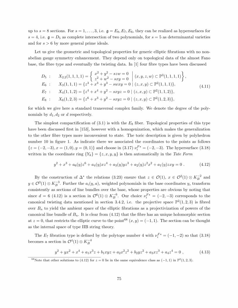
up to s = 8 sections. For s = 1, . . . , 3, i.e. g = E8, E7, E6, they can be realized as hypersurfaces for
s = 4, i.e. g = D5 as complete intersection of two polynomials, for s = 5 as determinantal varieties
and for s > 6 by more general prime ideals.
Let us give the geometric and topological properties for generic elliptic fibrations with no non-
abelian gauge symmetry enhancement. They depend only on topological data of the almost Fano
base, the fibre type and eventually the twisting data. In [1] four fibre types have been discussed
D5 : X2,2(1, 1, 1, 1) =
x2 + y2 − szw = 0z2 + w2 − sxy = 0
∣∣∣∣ (x, y, z, w) ⊂ P3(1, 1, 1, 1)
,
E6 : X3(1, 1, 1) = z3 + x3 + y3 − swxy = 0 | (z, x, y) ⊂ P2(1, 1, 1),
E7 : X4(1, 1, 2) = z4 + x4 + y2 − sxyz = 0 | (z, x, y) ⊂ P2(1, 1, 2),
E8 : X6(1, 2, 3) = z6 + x3 + y2 − sxyz = 0 | (z, x, y) ⊂ P2(1, 2, 3),
(4.11)
for which we give here a standard transversal complex family. We denote the degree of the poly-
nomials by d1, d2 or d respectively.
The simplest compactification of (3.1) is with the E8 fiber. Topological properties of this type
have been discussed first in [153], however with a homogenization, which makes the generalization
to the other fibre types more inconvenient to state. The toric description is given by polyhedron
number 10 in figure 1. As indicate there we associated the coordinates to the points as follows
z = (−2,−3), x = (1, 0), y = (0, 1) and choose in (3.17) νF∗i = (−2,−3). The hypersurface (3.18)
written in the coordinate ring Yk = z, x, y, u is then automatically in the Tate Form
y2 + x3 + a6(u)z6 + a4(u)xz4 + a3(u)yz3 + a2(u)z2x2 + a1(u)zxy = 0 . (4.12)
By the construction of ∆∗ the relations (3.23) ensure that z ∈ O(1), x ∈ O2(1) ⊗ K−2B and
y ∈ O3(1)⊗K−3B . Further the ai(u, a), weighted polynomials in the base coordinates u, transform
consistently as sections of line bundles over the base, whose properties are obvious by noting that
since d = 6 (4.12) is a section in O6(1) ⊗ K−6B . Our choice νF∗i = (−2,−3) corresponds to the
canonical twisting data mentioned in section 3.4.2, i.e. the projective space P2(1, 2, 3) is fibred
over Bn to yield the ambient space of the elliptic fibrations as a projectivization of powers of the
canonical line bundle of Bn. It is clear from (4.12) that the fibre has an unique holomorphic section
at z = 0, that restricts the elliptic curve to the point68 (x, y) = (−1, 1). The section can be thought
as the internal space of type IIB string theory.
The E7 fibration type is defined by the polytope number 4 with νF∗i = (−1,−2) so that (3.18)
becomes a section in O4(1)⊗K−4B
y2 + yx2 + x4 + a1x3z + b1xyz + a2x
2z2 + b2yz2 + a3xz
3 + a4z4 = 0 , (4.13)
68Note that other solutions to (4.12) for z = 0 lie in the same equivalence class as (−1, 1) in P2(1, 2, 3).
75
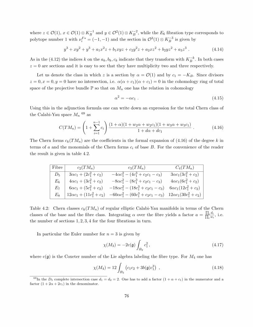
where z ∈ O(1), x ∈ O(1)⊗K−1B and y ∈ O2(1)⊗K−2
B , while the E6 fibration type corresponds to
polytope number 1 with νF∗i = (−1,−1) and the section in O3(1)⊗K−3B is given by
y3 + xy2 + y3 + a1x2z + b1xyz + c2y
2z + a2xz2 + b2yz
2 + a3z3 . (4.14)
As in the (4.12) the indices k on the ak, bk, ck indicate that they transform with K−kB . In both cases
z = 0 are sections and it is easy to see that they have multiplicity two and three respectively.
Let us denote the class in which z is a section by α = O(1) and by c1 = −KB. Since divisors
z = 0, x = 0, y = 0 have no intersection, i.e. α(α+ c1)(α+ c1) = 0 in the cohomology ring of total
space of the projective bundle P so that on Mn one has the relation in cohomology
α2 = −αc1 . (4.15)
Using this in the adjunction formula one can write down an expression for the total Chern class of
the Calabi-Yau space Mn69 as
C(TMn) =
(1 +
n−1∑i=1
ci
)(1 + α)(1 + w2α+ w2c1)(1 + w3α+ w3c1)
1 + dα+ dc1. (4.16)
The Chern forms ck(TMn) are the coefficients in the formal expansion of (4.16) of the degree k in
terms of a and the monomials of the Chern forms ci of base B. For the convenience of the reader
the result is given in table 4.2.
Fibre c2(TMn) c3(TMn) C4(TMn)
D5 3αc1 + (2c21 + c2) −4αc2
1 − (4c31 + c2c1 − c3) 3αc1(3c2
1 + c2)
E6 4αc1 + (3c21 + c2) −8αc2
1 − (8c31 + c2c1 − c3) 4αc1(6c2
1 + c2)
E7 6αc1 + (5c21 + c2) −18αc2
1 − (18c31 + c2c1 − c3) 6αc1(12c2
1 + c2)
E8 12αc1 + (11c21 + c2) −60αc2
1 − (60c31 + c2c1 − c3) 12αc1(30c2
1 + c2)
Table 4.2: Chern classes ck(TMn) of regular elliptic Calabi-Yau manifolds in terms of the Chern
classes of the base and the fibre class. Integrating α over the fibre yields a factor a =∏i di∏i wi
, i.e.
the number of sections 1, 2, 3, 4 for the four fibrations in turn.
In particular the Euler number for n = 3 is given by
χ(M3) = −2c(g)
∫B2
c21 , (4.17)
where c(g) is the Coxeter number of the Lie algebra labeling the fibre type. For M4 one has
χ(M4) = 12
∫B3
(c1c2 + 3b(g)c3
1
), (4.18)
69In the D5 complete intersection case d1 = d2 = 2. One has to add a factor (1 + α+ c1) in the numerator and afactor (1 + 2α+ 2c1) in the denominator.
76

with b(D5) = 1, b(E6) = 2, b(E7) = 6 and b(E8) = 10. We note here that this result of the discussion
is already summarized in figure 1 where we indicate on each point of the fiber polynomial the data
c(g)/36b(g) : h11(Pn−1)(htwist11 (Pn−1)) . (4.19)
Independent of the Lie algebra meaning c(g) and 36b(g) denotes just the coefficient in (4.17,4.18)
and h11(Pn−1) denotes the number of h11 for the basis Pn−1, while htwist11 + 1 denotes the number of
irreducible components of z = 0 hyperplane. In the special class of Calabi-Yau n-folds the C.T.C
Wall data that specifies the topological type of Mn and even the quantum cohomology can be fixed
from base and fibre data. On the other hand starting from the generic model it is possible to specify
the corrections to (4.18) and the other mentioned data due to singular fibres.
5 Compact Calabi-Yau manifolds with gauge groups
Here we discuss first the non-abelian gauge symmetry enhancements that follows from the Kodaira
classification [154][155] and monodromy data that can be obtained for the E8 fibre from the Tate
algorithm [156][35][157].
Further global gauge U(1) gauge symmetry enhancement come from additional global sections
of the elliptic fibre as was predicted in [18], explicitly constructed in [65] and interpreted in the
heterotic limit as split spectral cover in [158].
We argue that the loci of enhanced gauge symmetry corresponds to sub-monodromy problems
in the complex moduli space that can hence be reached by turning on the corresponding fluxes on
the vanishing periods.
5.1 Non-abelian gauge symmetries
Gauge symmetry enhancements are obtained by specializing the complex structure in the generic
clean sheet model so that the local behaviour of the base and moduli dependent coefficients in the
elliptic fibre, which are given for the (E8, E7, E6) fiber types in (4.12,5.23,5.27), near a given divisor
Dg in the base is of the desired form. The non-abelian gauge group G follows from
• g1) The Kodaira singular fibre type, which is specified by the Weierstrass data [f, g,∆ = f3−27g2] according to Kodaira’s classification reproduced in table A.1. The Weierstrass data are
obtained using Nagells algorithm and are given for the (E8, E7, E6) fibres in (5.2,5.25,5.30)70
70One can take any of the 2d reflexive polyhedron in figure 1 as fibre polytope and obtain their Weierstrass datafrom trivial specializations of the Newton polynomial for the polyhedra 10 (E8), 13 (E7), 15 (D5) and 16 (E6). TheWeierstrass data of polyhedra 10, 13, 15 and 16 are given in appendix A of [53].
77
• g2) The possible monodromy in Dg acting by an automorphism on the homology of the fibre.
This reduces the Lie algebra g of the Kodaira type to a non simply laced one with lower rank:
Z3 : D4 → G2, Z2 : E6 → F4, Z2 : Dn → Bn−1 , Z2 : A2n+1 → Ck.
For the E8 fibre Tate’s algorithm relates the monodromies to the leading coefficients in the Tate
form (4.12) that vanish generically in codimension one in Bk>1 [156][35][157], summarized in table
A.2 and A.3. Higher codimension singularities occur if the divisors Dg are singular or cross each
other and have not been treated systematically.
If we consider toric divisors Dg, the specialization of the complex structure amounts to set ai in
(3.18) to zero, i.e. to exclude points νi1 , . . . , νis of ∆. This reducesMcs to a monodromy invariant
subspace S if ∆ = 〈∆ \ νi1 , . . . , νis〉 ⊂ ΓR is a reflexive polyhedron in the reduced lattice Γ. This
implies that ∆∗ ⊂ Γ∗R exists and resolves the singularities of W∆ = 0 torically. As we argued in the
previous sections that implies the gauge symmetry enhancement occurs at the minimum of a flux
superpotential.
For the clean sheet models the coefficients of the fibrations are usually generic enough so that
if one enforces vanishing orders of [f, g,∆] at a single divisor for a low rank gauge group, the
change of the Hodge number ∆(h11) in the torically resolved model is entirely due to homological
non-trivial71 divisors of the form of a P1 fibration over Dg, where the P1 are the blow ups of the
Kodaira singularity, whose intersections yield then the negative Cartan matrix of g. In particular
∆(h11) = rank(g) and this information combined with the original Kodaira singularity type fixes
the possible outer automorphism.
Of course if the rank of the gauge group exceeds a bound the polyhedron ceases to be reflexive
and if one approaches this bound from below the coefficients of the corresponding fibre types are not
generic enough so that the toric resolution produces in addition to the gauge divisors, exceptional
divisors, whose shrinking lead e.g. to tensionless strings. For example at a single toric divisor in a
clean sheet model with fibre type En leading to a 6d or 4d theory it is not possible to enhance the
singularity just to En. Similarly we have studied intersecting toric gauge divisors in the base. It is
possible to enforce low rank gauge groups on three intersecting divisor and just get the exceptional
divisors that correspond to the gauge symmetry enhancements including the standard model gauge
group, but as expected higher rank groups on intersecting divisors produce additional singularities.
For the E8 fiber we choose a construction with heterotic duals and investigate the effects of
non-generic coefficients for the resolution of higher rank gauge groups in A.1 as compared to the
generic Tate algorithm. For the 4-fold B2 is determined by the polytopes of Figure 1 such that
B3 = P1 × B2 and for the 3-fold case the base is given by B2 = P1 × P1. One finds that even in
the most generic global models the coefficients are usually less generic than assumed in local model
building.
71I.e. the eventual outer automorphism is already divided out in the global toric construction.
78

As mentioned the E7 (5.23), E6 fibre (5.27) and D5 fibre [53] can be locally brought into
Weierstrass form using Nagells algorithm, see (5.25,5.30) and [53]. This information, i.e. the
vanishing orders of [f, g,∆] at Dg gives the Kodaira fibre type over the generic point in Dg that
yields the upper bound on the rank of the gauge group. Often one can understand the additional
effects due to the non-generic coefficients and using ∆(h11) from the toric resolution one can fix
the outer automorphism. One can then turn Nagells formalism around and specify similarly like
in table A.2 and A.3 the leading behaviour of the coefficients in (5.23,5.27) that leads to the
desired gauge group, see tables A.6 and A.7. This reproduces the results obtained from the “tops”
introduced in [159] and used in [160] in the same context, but is slightly more general, because it
is not restricted to the toric embeddings and also applies to crossing toric divisors.
5.2 The E8 fibre and Tate’s algorithm
Since for the E8 fibre (3.18) is in the Tate form (4.12), which we reproduce for convenience
y2 + x3 + a6(u)z6 + a4(u)xz4 + a3(u)yz3 + a2(u)z2x2 + a1(u)zxy = 0 ,
one can restrict the complex structure moduli z 72 to achieve singular fibers at a given divisor in
the base. For example consider cases with a P1 fibration over a heterotic base Bn−2 and call the
coordinates Yk = z, x, y, u1, . . . um, w, v, where ui are now coordinates of the heterotic base
Bn−2 and w, v are homogeneous coordinates of the P1. E.g. for w = 0 the whole Bn−2 becomes a
gauge divisor Dg and by setting the coefficients of the monomials in ai(u, v, w, z) to zero. i.e. by
specializing the complex structure moduli, one can achieve that ai(u, v, w, z) are of the form
a1 = α1w[a0] , a2 = α2w
[a2] , a3 = α3w[a3] , a4 = α4w
[a4] , a6 = α6w[a6] , (5.1)
where αi(u, v, w, z) are of order zero in w. Choosing this leading behaviour at w = 0 or at any
other divisor Dg of the base Bn−1 leads by Tate’s algorithm to singular fibres and hence a gauge
group along Dg. The association of the leading powers of [ai] with the singularity is given by Tate’s
algorithm [156], which is reproduced in [35]. The Kodaira type follows already from the Weierstrass
data (3.1) [f, g,∆ = f3 − 27g2], which we give for completeness
f =(a2
1 + 4a2
)2−24(a1a3+2a4), g =1
332
(36(a1a3+2a4)(a2
1 + 4a2
)−216
(a2
3 + 4a6
)−(a2
1 + 4a2
)3) .
(5.2)
5.2.1 The stable degeneration limit and the moduli space of the central fibre
We demonstrate the formalism of landscaping by fluxes and the occurrence of the sub-monodromy
problem with the enforcement of the stable degeneration limit in the generic clean sheet elliptic
72From now on we use zi instead of ai to denote the complex structure variables, to avoid confusion with theai(u, v, w, z), which are moduli dependent sections over the base. Coordinates on the base Bn−1 are denoted generi-cally by u, but if Bn−1 has a fibration structure P1 → Bn−2 we call the coordinates pf P1 v, w and the coordinatesof Bn−2 u .
79
K3, given by the member MA1 of the A-series X12(1, 1, 4, 6) considered in sect 5.3.3. In the eight
dimensional case the F-theory base is B1 = P1 parametrized by v, w while the heterotic base Bn−2 =
B0 = pt is trivial. However the essential features carry over to the situation when the P1 is a fibration
over B1 or B2. The polyhedron ∆∗ is defined by the points 1,−2,−3,−1,−2,−3,0,−2,−3′,0, 1, 0, 0, 0, 1 corresponding to coordinates v, w, z, x, y. Of course ∆∗ contains the inner point
ν∗0 and the points above are corners except for the primed one, which it lies on an edge. The section
of the anti canonical bundle characterizing the K3 defined by (3.18) reads
W∆ = y2 + x3 + (a1v12 + a2v
11w + a3v10w2 + a4v
9w3 + a5v8w4 + a6v
7w5 + a7v6w6+
a8v5w7 + a9v
4w8 + a10v3w9 + a11v
2w10 + a12vw11 + a13w
12)z6 + (a14v8 + a15w
8)xz4+(a16v
6 + a17w6)yz3 + (a18v
4 + a19w4)z2x2 + a20(vw)xyz .
(5.3)
From the 20 ai, two are redundant, but we keep the full flexibility to set them to zero and impose
Kodaira fibres at v = 0 and (or) at w = 0 using (5.1). Passing from the restricted polynomial
to its Newton polytope and checking whether the restricted polytope is reflexive yields the sub-
monodromy problems related to the gauge groups at v = 0, w = 0 of the elliptic K3 hypersurface in
this toric ambient space. In particular we can enforce two E8 fibres at w = 0 and v = 0. This adds
16 points to ∆∗ to complete the polytope∆∗
= 6,−2,−3,−6,−2,−3,0,−2,−3′, 0, 1, 0,0, 0, 1, see [159][20][161] for explicit lists of these points. The 16 new points correspond to the
toric resolution of the two E8’s. The restricted polynomial is
W ∆
= a1y2 + a2x
3 + a3v7w5z6 + a4v
5w7z6 + a5v6w6z6 + a0vwxyz . (5.4)
It is combinatorial equivalent to the invariant polynomial under the maximal phase symmetry group
Z2 × Z3 generated by (y → −y, v → −v) and (x→ exp(2πi/3)x, v → exp(−2πi/3)v)
W ∆ph
= a1y2 + a2x
3 + a3v12z6 + a4w
12z6 + a5v6w6z6 + a0vwxyz , (5.5)
in the coarse invariant latticeΓph. In either formulation of the restriction one uses the arguments
given before, to conclude that there is the heterotic G-flux in F-theory, which drives the complex
moduli in the fibred 4d version to the stable degeneration limit. The Gauss-Manin connection for
the sub-monodromy problem is readily obtained using GGKZ method described in section (3.7).
It depends on the linear relations among the points of the Newton polyhedron, which are
l(e) = (−6, 3, 2, 0, 0, 1), l(b) = (0, 0, 0, 1, 1,−2) , (5.6)
where l(e) is the Mori vector associated to the elliptic fibre class, while l(b) is associated to the
base class. This leads straightforwardly [83] to the Picard-Fuchs differential ideal IPF of the sub-
monodromy problem of the central fibre generated by
D1 = θe(θe − 2θ2)− 12ze(6θe + 5)(6θe + 1), D2 = θ2b − zb(2θb − θe)(2θb − θe + 1) . (5.7)
80

According to [18] (see also the discussion [23]) the stable degeneration is where the Kahler class ρ
in the dual heterotic string is large ρ→ i∞, while the complex structure of the F-theory torus τ is
identified with the complex structure of the heterotic torus τ . The sub-monodromy problem was
solved in [162]. In fact in an elliptically fibred 3-fold with B1 = P1, which has a heterotic dual,
in the eight dimensional limit vol(B1) → ∞. The equivalence is immediate by noticing that (5.7)
is equivalent to the first two differential operators in eq. (9) in [162], which determine the finite
periods in the eight dimensional limit. Hence the map from the F-theory moduli to the heterotic
theory is completely precise and one can identify the stringy gauge theory enhancements of the
heterotic T2 compactifications in the F-theory moduli space. It is fixed by the modular properties
of the mirror map and given in [162] as
ze =j(τ) + j(ρ)− µ
j(τ)j(ρ) +√j(τ)(j(τ)− µ)
√j(ρ)(j(ρ)− µ)
,
zb = 2
[j(τ)j(ρ) +
√j(τ)(j(τ)− µ)
√j(ρ)(j(ρ)− µ)
]2j(τ)j(ρ)[j(τ) + j(ρ)− µ]2
,(5.8)
where µ = 1728. Calculating the discriminant of (5.4) yields after some scaling δ1 = (1− 4zb) and
δ2 = (1−432ze)2−1728z2
ezb. Comparing with heterotic string at δ1 = 0 one has at ρ = τ an SU(2)
enhancement while for δ2 = 0 we have solutions ρ = τ = i corresponding to the SU(2)×SU(2)- and
at ρ = τ = exp(2πi/3) to an SU(3) stringy heterotic gauge theory enhancement [162]. Specializing
the complex structure to get the E8 Kodaira singularities at antipodal points of the base P1 is the
first step to reach the stable degeneration limit. In addition one has to chose the volume of the
base P1 to be infinite, which according to (5.6) means zb = 0. As explained in some detail in [23]
in complex geometry this means that the base P1 splits into two Hi ∼ P1i , i = 1, 2, which share one
common point Q. One has π−1(Q) = T 2het and π : E → Hi are two rational elliptic surfaces. Since
they have 4 I1 fibres and one E8 Kodaira fibre or at more generic points in their complex structure
moduli space 12 I1 fibers they are called 12K3. Hi is a section of the corresponding elliptic fibration
with projection map π. Blowing down this section yields an dP8 del Pezzo surface obtained by
eight successive blow ups of P2. Instead of an elliptic fibration the dP8 is an elliptic pencil with a
base point. Blowing up the latter gives back the 12K3, which maybe also called dP9.
The map (5.8) describes precisely how the limit decompactifies the elliptic torus, since ρ→ i∞(j(ρ) → ∞) corresponds to zb → 0, while ze = 1
j(τ)+√j(τ)(j(τ)−µ)
is the map to the complex
structure modulus of heterotic torus in the stable degeneration limit. The map distinguishes the 2
moduli of the central fibre, the heterotic T 2het whose sub-monodromy system we solved above, from
the 16 moduli of the heterotic E8 × E8 bundle, whose sub-monodromy system is discussed in the
next section.
81

5.2.2 The moduli space of gauge bundles and the [p, q] string states of E8 gauge group
For the E8 fibre type compactified in a toric ambient space the following data describe equivalently
the gauge theory enhancement with gauge group G over a codimension one toric divisor Dg in the
base Bn−1, n > 2:
• G1) The classification of the Kodaira fibre types and the action of monodromies in Dg on its
homology as encoded in the vanishing order of the coefficients [a0, a2, a3, a4, a6] of the Tate
form at the divisor Dg.
• G2) The “tops” classified in [159] constructed torically over Dg.
Simply restricting the coefficients of the Tate form W∆ → W ∆
and constructing∆∗
yields the
additional points in “tops” as embedded 73 in∆∗, which are listed in [159][20][161]. In the special
case of a P1 fibration over Bk with (v : w) homogeneous coordinates of the fibre P1 one gets the
“tops” by restricting the coefficients of the Tate form near v = 0 and the “bottoms” by restricting
them near w = 0. This was used e.g. in [20] to construct the same heterotic gauge group in each
of the heterotic E8 to get a Z2 symmetric model that allows for a CHL involution.
As mentioned for high rank gauge groups close to the bound of non-reflexivity the additional
effects due to non-generic coefficients in the compactification is not systematically explored and
the information G1) is more universal as it can be immediately used to construct gauge groups on
crossing toric and non-toric divisors.
Taking the stable degeneration limit described in the last section in the cases with heterotic
duals Zn−1 = (Ehet 7→ Bn−2), i.e. for F-theory bases of the form Bn−1 = (P1 → Bn−2), one gets the
maps from the heterotic bundle moduli to the F-theory moduli [23]. For each heterotic elliptic fibre
E = Ehet the moduli space of the holomorphic G-bundle is described by the moduli space of the map
from the weight lattice Γg of G to the Jacobian of E modulo the Weyl group φ : Γg → Jac(E)/Weyl,
see e.g. [163]. This moduli space is a weighted projective space Pr(s0, . . . , sr), where r is the rank
and si are the Coxeter numbers of G [164]. This description can be fibred over the base and except
for the gauge group G = E8 the moduli of G-bundles on the elliptically fibred Calabi-Yau manifold
Zn−1 are described by a projectivization W of the bundle O ⊕ (⊕ri=1L−di) over Bn−2. Here L−1
is the normal bundle of the base and di are the degrees of the independent Casimir operators of
G. For n ≤ 3 the G-bundle can be reconstructed from a section of s : Bn−2 → W, which is called
spectral cover C of B and a line bundle on C, called S. E.g. for G = SU(N) the G-bundle on E is
given explicitly as V = ⊕ni=1Ni, where ⊗ni=1Ni = O, which implies that the Ni vanish of first order
at Qi and have a pole at the origin P , i.e. Ni = O(Qi)⊗O(P )−1, with∑n
i=1Qi = 0 in the group
73Constructing the additional points is part of the functionality of Sage [77]. We wrote a code, which is based upona mathematica program that P. Candelas released some 12 years ago.
82

law in E . On E = X6(2, 3, 1) with coordinates x, y, z and z = 0 is P such points are specified by
the spectral equation
w = a0 + a2x+ a3y + a4x2 + . . .+
an−1x
N/2 n even
an−1yx(N−3)/2 n odd .
(5.9)
Let us take the coordinates for ∆∗ as in the previous section. The identification of the moduli is
discussed in [161] and amounts to change the identification of the C∗ actions in order to define P∆ in
the limit. Define the coordinate ring of the dual space by (1, 0, 0) ∼ x1 =: v, (0,−1,−1) ∼ x2 =: z,
(0, 2,−1) ∼ x3 =: x and (0,−1, 1) ∼ x4 =: y. This allows to write W∆∗ in the limit as follows [161]
WBM∆∗ = w0(x, y, z, u) + w− + w+ with
w− =
J∑j=1
vjwj−(x, y, z, u), w+ =
J∑j=1
v−jwj+(x, y, z, u),(5.10)
where the monomials Mi of WBM∆∗ are defined by Mi =
∏j x〈ν∗i ,νj〉+1−δj,1j . Because of the shift
δ1,m, WBM∆∗ = 0 is not quite the correct global description of Wn as it tempers with scalings on
the P1, which is the base of the elliptic fibration, but as long as one focusses on the north- or on
the southpole of the (fibre) P1 , e.g. by scaling wj− → εjwj− and sending ε → 0, one can extract
the local limit for patch v 6= 0. The logic is [165] that as long as the exponents of the (Laurant)
monomials of the Newton (Laurant) polynomial obey the linear relations described by the charge
vectors l(i) ∏l(i)j >0
Ml(i)j
j =∏l(i)j <0
Ml(i)j
j , ∀ j , (5.11)
which implies that the periods of that geometry are annihilated by the (3.49) operator, the B-model
geometry of the local sub-monodromy problem is captured faithfully by that Newton (Laurant)
polynomial. Moreover by the fibration structure of the base P1 → Bn−2, w0(x, y, z, u) = 0 is an
elliptic fibration in the Tate form over Bn−2, which is the heterotic Calabi-Yau Zn−1. In the limit
for n = 2 one gets e.g. for SU(N), where we neglected in w0 the points on codim 1 faces,
WL = (y2+x3+z6+αxyz)+v
(a
(1)0 zN + a
(1)2 xzN−1 + a
(1)3 yzN−2 + . . .+
a
(1)n−1x
N2 neven
a(1)n−1yx
N−32 n odd
).
(5.12)
For SU(N) v appears only linearly and one can argue that the linear v can be integrated out to
one is left with w0(x, y, z) = 0 and w1+ = 0. This is the same information as in (5.9) and is easy
to see that the weights si of the a(si)i over the base are given by the power si of vsi multiplying
them. In the polyhedra language this is the height of the additional point. The case with the most
different heights is the E8 case which are the same than in an E8 del Pezzo with fixed canonical
section with weights fitting into P8(1, 2, 2, 3, 3, 4, 4, 5, 6)
w1+ = a
(1)1 z5, w2
+ = a(2)1 z4 + a
(2)2 x2 w3
+ = a(3)1 z3 + a
(3)2 y
w4+ = a
(4)1 z2 + a
(4)2 x, w5
+ = a(5)1 z w6
+ = a(6)1 .
(5.13)
83
This geometry i.e. an elliptic curve E given by the fixed anti-canonical bundle in an E8 del Pezzo
surface S was used by Looijenga [163] to describe the E8 gauge bundle on E . Let −K = c1(TS)
and L = H2(S,Z), then the orthogonal lattice L′ ∈ L with L′ ·K = 0 is the weight lattice of E8
(which is isomorphic to the root lattice as the E8 lattice is selfdual). As explained in [163][23]
every y ∈ L′ gives rise to a line bundle on S whose restriction to E yields the desired map from
the weight lattice to the Jacobian of E modulo the Weyl transformation. By the Torelli theorem
the moduli of that map are the moduli of the pair (E , S), i.e. a projectivization of the parameters
in (5.13).74 Note that the dual polynom W∆∗ enters that construction. This follows from mirror
symmetry on the K3, which exchanges the horizontal- and the vertical subspaces of the cohomology.
In the polarization that is fixed by the toric embedding of Mn in P∆∗ and Wn in P∆ these spaces
determine, which gauge groups G and H can be enhanced by specializing the Kahler moduli and
the complex moduli respectively. The groups G and H are exchanged by exchanging Mn with
Wn [166][167][168]. A list of the groups H and G for those K3 polyhedra that realize the Tate
degenerations is given in [161].
Instead of looking at the del Pezzo surfaces it is better to start with the half K3, which contains
all del Pezzo surfaces as blow down limits. This geometry has an elliptic fibration, and geomet-
rical invariants associated to curves in it have a very nice relation to the affine E8 group. The
latter appears also in the work of [163] and has been extended from Loop groups to torus groups
in [169]. For smooth elliptic fibrations the genus g instanton generating function can be organized
as follows [170]
Fg(q,Q) =∑
β∈H2(Bn−1,Z)
(q
124
η(q)
)p(β)
Pp′(g,β)(E2, Gw1 , . . . , Gwd)Qβ, (5.14)
where β is the base degree and Qβ = exp(2πi∑
k βktk) with tk, k = 1, . . . , h11(Bn−1) are the Kahler
classes of the basis, while the fibre degree is encoded in q = exp(2πiτ), where τ is the dilaton, and
given by the Fourier expansion of the modular functions and form. In particular η(q) is the Dedekind
η-function, E2 is the second Eisenstein series and Gw1 , . . . , Gwd are the generators of the modular
forms associated to the elliptic fibre type. They depend on the number of torsion points and hence
the number of sections of the elliptic fibration. p, p′ are linear in their arguments with coefficients
spelled out for general basis in [170]. The structure was first observed for rational elliptic surfaces
in [65] [171][172]. If the latter have the E8 fibre type, currently under discussion, there are only
no additional torsion poinst and the modular group is PSL(2,Z) with the two generators G4 = E4
and G6 = E6. For rational surfaces Bn−1 = P1 with one class β and p = 12β and p′ = 2g− 2 + 6β.
In this case
F0(q,Q) =q
12E4
η12(q)Q+
q(E2E24 + 2E4E6)
24η24(q)Q2 +O(Q3) , (5.15)
74To see that the form of the del Pezzo surface and E given in [23] is equivalent to (5.13), identify the u used [23]with the v used here and identifications of the deformations modulo the ideal ∂xWL, ∂yWL∂zWL, which do respectthe scaling in P8(1, 2, 2, 3, 3, 4, 4, 5, 6).
84
is the genus zero prepotential. One can get this result from a sub-monodromy system in an elliptic
Calabi-Yau 3-fold. As in the previous section it is trivial to embed it in a 4-fold geometry e.g. by
fibering the 3-fold over P1. The reason that one starts with a 3-fold rather than describe the two
dimensional geometry directly as for the K3 in previous section is that the half K3 has positive
Chern class. Hence we have to consider the non-compact total 3d space O(−K 12K3) → K 1
2K3, i.e.
the canonical line bundle over the half K3. 3-folds with such a local limit are elliptic fibrations
with E8 fibre type, i.e. ∆∗F2 = ∆(10)2 with ν∗F = (−2,−3) over the Hirzebruch surface F1 = P
∆(3)2
with the 2d polyhedra in figure 1. Hence the relevant points for the polyhedron ∆∗ are
ν∗i l(e) l(b) l(f)
x0 0 0 0 0 −6 0 0u1 1 0 −2 −3 0 1 0u2 −1 0 −2 −3 0 1 −1w 0 1 −2 −3 0 0 1v −1 −1 −2 −3 0 0 1z 0 0 −2 −3 1 −2 −1x 0 0 1 0 2 0 0y 0 0 0 1 3 0 0
(5.16)
and the l(i) vectors generate the Picard-Fuchs ideal IPF
D1 = θe(θe − 2θb − θf )− 12ze(6θe + 5)(6θe + 1) , (5.17)
D2 = θb(θb − θf )− zb(2θb + θf − θe)(2θb + θf − θe + 1) , (5.18)
D3 = θ2f − zf (θf − θb)(2θb + θf − θe) . (5.19)
From the last section we know that l(e) and l(b) correspond to the moduli of the central fibre and that
the stable degeneration limit is zb → 0 or equivalently that the volume of the base of the elliptic K3
is taken to infinity. In this limit it is more non-trivial to obtain the sub-mondromy system, as the
invariant point configuration is not reflexive, but corresponds rather to the non-compact CY 3-fold.
From the Picard-Fuchs ideal of the local system it can be proven that the period F0 is expressible
in terms of the modular forms, see [172] for the E6- and [170] for the E8 fibre type. Because of
the map (4.9) the specialization of the global Calabi-Yau Picard-Fuchs system only captures two of
the 10 parameters of the half K3, the base with parameter Q and the fibre with parameter q. The
moduli parametrizing the E8 vector bundle can be added using the Weyl symmetry [171]. There
are nine Weyl invariant Jacobi forms for the E8 lattice Ai, i = 1, . . . , 5 and B2, B3, B4 and B6, the
simplest being A1 = Θ(~m, q)~m=0 = E4
ΘE8(~m, τ) =∑~w∈Γ8
eπiτ ~w2+2πi~m·~w =
1
2
4∑k=1
8∏j=1
θk(mj , τ) =∑Op,k
qp∑
~w∈Op,k
e2πi~m·~w, (5.20)
85

and transforms with weight four and index one 75. Here Op,k are the Weyl orbits. In terms of the
nine forms the genus zero F0 prepotential can be written as
F0(q,m,Q) =q
12A1
η12(q)Q+
q(4E2A21 + 3A2E6 + 5E4B2)
96η24(q)Q2 +O(Q3) . (5.21)
The first observation is that the leading term is the superpotential of [4] 76. The minima of the
superpotential at dΘE8 = ΘE8 = 0 were determined in [4]. The conclusion is that the moduli q
and Q are not restricted, but that the minima are at common zeros of the θk(mj , τ). Because of
the K3 mirror duality exchanging G and H one can view this superpotential also as prepotential
of the complex moduli problem of the generic K3 discussed in the last section near one tip of the
P1. The fact that F0 does not obstruct q and Q is in perfect agreement with the analysis of the
last section, where q and Q become the unobstructed moduli of the central fibre.
The analysis of this section recalls how to identify the bundle moduli in F-theory so that the
flux superpotential and the metric can be evaluated for these moduli, with the formalism developed
in the previous section.
A maybe more exciting and mysterious aspect that shows up in this calculations is that the
superpotential or more generally the periods “count something”, when expressed in the correct
N = 1 variables. For example the leading term of (5.21) counts the rigid −2 curves (and thereby
the rigid divisors in M4) in the E8 del Pezzo, in other limit it counts disk instantons[5][10][11][12]
or D-instantons[6]. The structure becomes even more interesting, when one includes higher genus
invariants. The most information one gets out, when one uses the refined counting that splits the
genus in two counting parameters introduced by Nekrasov. The refined invariants are labeled by
two spins jL/jR and for the half K3 they where obtained in [53] and interpreted as the states
associated to the [p, q] strings. For example for Qd=1 one gets:
2jL\2jR 0 1
0 248
1 1
d = 1
and in particular the 248 in this expression have been interpreted as the ground state of the
[p, q] of the 7-branes with mutually non local charges that appear in the II∗ Kodaira fibre. The
splitting of the E8 representations of the genus one invariants into E8−k × U(1)k will be discussed
in the next section.
75For the other Weyl invariant Jacobi forms see e.g. [170].76In fact after a correction in the power of η that was found in [173], which does not invalidate the minimization
conditions stated in [4] .
86

5.3 Additional sections and additional U(1)
Let us point out the relation between the existence of k+ 1 global sections of the elliptic fibre and
the globalization of the abelian U(1)k that emerge in the Wilson line breaking of the E8 gauge
group to E8−k × U(1)k [65].
Let us look at one half K3 that arrises in the stable degeneration limit. All exceptional divisors
Ei, i = 1, . . . , 9 with intersection EiEj = −δij in d9P2 become sections of the elliptic fibration of
the rational elliptic surface. This can be seen as follows. The elliptic fibre class is e = −K =
3H −∑9
i=1Ei, where H is the hyperplane class of P2. Using H2 = 3 and HEi = 0 one gets e2 = 0,
i.e. the section of the anti-canonical bundle, which is always an elliptic curve, becomes now a fibre,
and Ei intersect the fibre with eEi = 1 are now sections of the fibration. If we consider the stable
degeneration that arises in elliptic fibrations over F1 one gets the situation depicted in figure 2.
Figure 2: Stable Degeneration limit of a heterotic fibration
If we smooth the geometry to the generic fibration with E8 fibre type over F1 the co-kernel of
the map i∗ : H2(Mn) 7→ H2(S) is eight dimensional and one has only the fibre e and the zero section
f represented in the Calabi-Yau Mn. As was explained in [18] one can flop the zero section by a
transition to a second phase, which is described at the level of the Mori cone by l(1) = l(e) + l(f),
l(2) = l(b) + l(f) and l(3) = −l(f). This flops out the P1 or a ruled divisor in the higher dimensional
case, which corresponds to the zero section. This makes the half K3 into the d8P2 del Pezzo. The
latter can be shrunken in an extremal transition to an elliptic fibration over P2 [18]77. If one wants
to globalize k more sections one has to use elliptic fibrations with k torsion points on which the red
and the green sections can be anchored. Such points occur in fibres with more symmetries namely
77 For n = 3 the transition is very well understood from the anomaly cancellation in the 6d effective theory. Itenforces a relation between number of hyper- vectors and tensor multiplets, which is H − V − T = 3 + c(g)(9− T ).The number of tensor multiplets is T = h11(B2)− 1 and for the clean sheets models V = (k− 1), H = h21(M3) + 1 aswell as h11(M3) = h11(B2) + (k + 1). In particular for k = 0 one has [18] c(g) = 30, which taking into account thatby Riemann-Roch for rational surfaces c21(B2) = 10− h11(B2), gives back (4.17). Similar matchings hold for generalk.
87
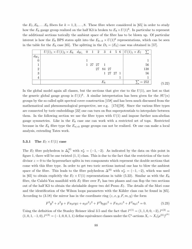
the E7, E6, . . . E0 fibers for k = 1, 2, . . . , 8. These fibre where considered in [65] in order to study
how the E8 gauge group realized on the half K3 is broken to E8×U(1)k. In particular to represent
the additional sections torically the ambient space of the fibre has to be blown up. Of particular
interest is how the E8 BPS states split into the E8−k × U(1)k representations, which can be seen
in the table for the E6 case [65]. The splitting in the D5 = (E5) case was obtained in [57].
U(1)1 × U(1)2 × E6 dW1 0 1 2 3 4 5 6 U(1)1 × E7∑
dW2
0 1 11 1 27 27 1 562 27 84 27 1383 1 27 27 1 564 1 1
E8∑
= 252 (5.22)
In the global model again all classes, but the sections that give rise to the U(1), are lost so that
the generic global gauge group is U(1)k. A similar interpretation has been given for the SU(n)
groups by the so called split spectral cover construction [158] and has been much discussed from the
mathematical and phenomenological perspective, see e.g. [174][59]. Since the various fibre types
are connected by toric embeddings [22] one can turn on flux superpotentials to interpolate between
them. In the following section we use the fibre types with U(1) and impose further non-abelian
gauge symmetries. Like in the E8 case one can work with a restricted set of tops. Restricted
because in the Ek fibre type the En>k gauge groups can not be realized. Or one can make a local
analysis, extending Tates work.
5.3.1 The E7 × U(1) case
The E7 fibre polyhedron is ∆(4)2 with n∗F = (−1,−2). As indicated by the data on this point in
figure 1, there will be one twisted (1, 1) class. This is due to the fact that the restriction of the toric
divisor z = 0 to the hypersurface splits in two components which represent the double sections that
come with this fibre type. In order to get two toric sections instead one has to blow the ambient
space of the fibre. This leads to the fibre polyhedron ∆(6) with n∗F = (−1,−2), which was used
in [65] to obtain explicitly the E7 × U(1) representations in table (5.22). Similar as with the E8
fibre, the Calabi-Yau manifold with E7 fibre over F1 has two phases and can flop the two sections
out of the half K3 to obtain the shrinkable degree two del Pezzo E7. The details of the Mori cone
and the identification of the Wilson loops parameters with the Kahler class can be found in [65].
According to (3.18) the mirror has in the coordinate ring (z, x, y, F,m, u) the form
F 2y2 + x2y + Fa3xyz + a2x2z2 + F 2b2yz
2 + Fa1xz3 + F 2a0z
4 = 0. (5.23)
Using the definition of the Stanley Reisner ideal 3.5 and the fact that l∗(1) = (1, 1, 0, 0,−2), l∗(2) =
(1, 0, 1,−1, 0), l∗(3) = (−1, 0, 0, 1, 1) define equivalence classes under the C∗-actionsXi ∼ Xi(µ(k))l
(k)
88
one finds the single holomorphic section at h1 = (z = 0, x = 1, y = −1, F = 1).78 The second section
is at r1 = (z = 1, x = 1, y = −a2, F = 0). This is a rational section as the values of y depend of u
via a2(u). Note that (z = 1, x = 0, y = 1, F = 0) is in the Stanley-Reisner ideal.
The discriminant on the E7×U(1) fiber ∆ = f3− 27g2 is determined in terms of the functions
f and g given by
f =1
12(−24a1a3 + a4
3 + 8a23(a2 − b2) + 16(3a0 + a2
2 + a2b2 + b22)), (5.24)
g =1
216(−36a1a
33 + a6
3 − 144a1a3(a2 − b2) + 12a43(a2 − b2) + 24a2
3(3a0 + 2a22 − a2b2 + 2b22)
+ 8(27a21 + 8a3
2 − 36a0b2 + 12a22b2 − 8b32 − 12a2(6a0 + b22))).
For a 4-fold compactification, it is possible to chose B3 from 4319 different cases. To exemplify
we will choose the base B3 = P3 with coordinates ui, i = 1, 2, 3, 4, to write the codimension 1
enhancements appearing at a given vanishing order of one variable ui. The results are given in
Appendix A.2. Those tables also contain the codimension 1 singularities appearing in a 3-fold with
base B2 = P2 with coordinates ui, i = 1, 2, 3, at the point were a certain ui vanishes. Let us fix an
A4 singularity at u1 = 0, then for the A4 singularity the coefficients have the dependence
a3 = a3(ui) +Oa3(u1)fa3(ui), a2 = a2u21 +Oa2(u2
1)fa2(ui), b2 = b2u1 +Ob2(u1)fb2(ui),(5.25)
a1 = a1u21 +Oa1(u2
1)fa1(ui), a0 = a0u31 +Oa0(u3
1)fa0(ui).
The ak and b2 represent polynomials of ui which are different from zero when ui = 0, the f represent
polynomials on ui and the O(uj1) represent functions on higher order than j on u1. With the given
vanishing order of the coefficients at u1 = 0 the 3-fold has the properties: χ3 = −204, h311 =
7(0), h321 = 109(0) and for the 4-fold χ4 = 5898, h4
11 = 7(0), h431 = 968(0) and h4
21 = 0. As
mentioned, other enhancements for the bases B3 = P3 and B2 = P2 are summarized in appendix
A.2.
In our toric global construction it is possible to write models with different enhancements at
different divisors. Keeping for the 3-fold (4-fold) the base P2 (P3), one can set an SU(2) at u1 = 0
and an SU(3) at u2 = 0, with the following dependence of the coefficients
a3 = a3(ui) + Oa3(u1, u2)fa3(ui), a2 = a2(ui)u1u2 + Oa2(u1, u2)fa2(ui), (5.26)
b2 = b2(ui)u2 + Ob2(u01, u2)fb2(ui), a1 = a1(ui)u1u2 + Oa1(u1, u2)fa1(ui),
a0 = a0(ui)u1u22 + Oa0(u2
1, u1)fa0(ui).
The vanishing order can be checked in Table A.6 from appendix A.2. The ak, b2 represent poly-
nomials of ui which are different from zero when ui = 0, the f represent polynomials on ui and
78Note that z = 0 and W∆ = 0 implies F 2y2 +x2y = 0. The solutions of this equation could not be mapped to onepoint on the fibre without using the C∗-scaling that involves the coordinate associated to ν3. However this coordinatedoes not appear in W∆ = 0, because it can be eliminated by an automorphism of P∆∗ .
89

the O(ul1um2 ) represent functions on higher order than l on u1 and higher order of m on u2. For
the manifolds with bases P3 (P2) which accommodate those singularities we obtain the properties
χ4 = 5910, h411 = 6(0), h4
31 = 971(0) and h421 = 0 (χ3 = −210, h3
11 = 165(0) and h321 = 3(0)).
Let us consider one example with a different construction. Consider models with heterotic
duals, in which the base B3 is obtained as fibration of P1 over certain B2. We consider the case in
which B2 is generated by the polytope 7 in Figure 1, and there is no twisting thus B3 = P1 × B2.
In addition the 3-fold with heterotic dual is determined by the base B2 = P1 × P1. Let us localize
an A4 singularity at u1 = 0, the vanishing order for the coefficients is 0, 2, 1, 2, 3. In the 3-fold with
base B2 the properties are χ3 = −196, h311 = 8(0) and h3
21 = 106(0). For the 4-fold with base B3
the properties are χ4 = 4092, h411 = 11(0), h4
31 = 663(0) and h421 = 0.
Finally let us consider cases with heterotic duals in which the fibration is given by the vectors
ν(i)∗ ∈ ∆(i)∗B3 in (4.6), as well for polytope 7, and with twist m1 = −1, mi = 0, i = 2, ..., 6. The
properties of the 4-fold are given by χ4 = 3834, h411 = 11(0), h4
31 = 620(0), h421 = 0 .
5.3.2 The E6 × U(1)2 case
The fibre polyhedron with the triple section is ∆(1)2 with n∗F = (−1,−1) and two twisted (1, 1)
class, i.e. a triple section as indicated in figure 1. In order to get three toric sections and the
corresponding splitting of the instantons in E6 × U(1)2 the polyhedron ∆(5) has been considered
in [65], which leads by (3.18) in the coordinate ring (z, x, y, F,G, u) to
Gx2y+Fxy2 +G2a1x2z+FGb1xyz+F 2c1y
2z+FG2a2xz2 +F 2Gb2yz
2 +F 2G2a3z3 = 0 . (5.27)
Again the holomorphic section is at h1 = (z = 0, x = 1, y = 1, F = −G), while the rational ones
are at r1 = (z = 1, x = 1, y = −a1G,F = 0) and r2 = (z = 1, x = −b1F, y = 1, G = 0). Note
that the coefficients of x2y and xy2 transform in O of B. It has been noted in [59] that at the
expense of making all sections rational, one can allow the coefficients a0 and b0 instead to transform
a restricted set of ample line bundles over Bn.
On the E6 × U(1)2 fiber the functions which determine the discriminant ∆ = f3 − 27g2 are
given by
f =1
12(b41 − 8b21(a2 + b2 + a1c1) + 24b1(a3 + a1b2 + a2c1) + (5.28)
16(a22 − a2b2 + b22 − 3a3c1 + a2
1c21 − a1(3a3 + (a2 + b2)c1))) ,
(5.29)
90
g =1
216(b61 − 12b41(a2 + b2 + a1c1) + 36b31(a3 + a1b2 + a2c1) +
24b21(2a22 + a2b2 + 2b22 − 3a3c1 + 2a2
1c21 + a1(−3a3 + (a2 + b2)c1))−
144b1(a21b2c1 + (a2 + b2)(a3 + a2c1) + a1(b2(a2 + b2)− 5a3c1 + a2c
21))
−8(8a32 − 27a2
3 − 12a22b2 − 12a2b
22 + 8b32 + 18a3(a2 − 2b2)c1− 27a2
2c21 + 8a3
1c31 +
6a1(3a3(−2a2 + b2)− (2a22 + a2b2 + 2b22)c1 + 12a3c1
2)
−3a21(9b22 − 24a3c1 + 4(a2 + b2)c2
1))).
Let us now see the realization of codimension 1 singularities in the E6 × U(1)2 fiber. In table
A.7 we have given a list of singularities realized in the fiber with a given vanishing order for
the coefficients. In the table are also written the properties of a toric 3-fold (4-fold) constructed
using a base B2 = P2 (B3 = P3) in which the codimension 1 singularities are realized for a given
vanishing order of the coordinates ui, i = 1, ..., 3 ( i = 1, ..., 4). As an example let us look at the A4
singularity, which is one of the rows. The vanishing order for the variable u1 is given by 1, 0, 2, 1, 2, 2,
the properties of the 3-fold and 4-fold are respectively χ3 = −134, h311 = 8(0), h3
31 = 75(0), and
χ4 = 3168, h411 = 8(0), h4
31 = 512(0), h421 = 0.
Keeping the same basis for the 3-fold and 4-fold, let us impose an SU(2) singularity at u1 = 0
and an SU(3) singularity at u2 = 0. Consider the vanishing order for the coefficients 0, 0, 1, 0, 0, 1
at u1 = 0 and 1, 0, 1, 1, 1, 1 at u2 = 0. The properties of the 3-fold and 4-fold that embed the
mentioned singularities are given respectively by χ3 = −140, h311 = 7(0), h3
21 = 77(0) and χ4 = 3180,
h411 = 7(0), h4
31 = 515(0) and h421 = 0.
Let us look at an example where the 3-fold and 4-fold are constructed to accommodate heterotic
duals, B2 given by the polytope 7 of Figure 1, then B3 = P1 × B2. The B2 defining the 3-fold is
given by B2 = P1 × P1. The 4-fold (3-fold) will have an SU(5) singularity with vanishing order of
the P1 variable u1 given by 1, 0, 2, 1, 2, 2. The properties of the 3-fold will be χ3 = −128, h311 = 9(0),
h321 = 73(0), and the properties of the fourfold χ4 = 2226, h4
11 = 12(0), h431 = 351(0) and h4
21 = 0.
Let us look now at the case keeping B2 and constructing the base of the 4-fold as a fibration,
with a defined twist B3 = P1 → B2. The fibration is chosen to be the same as in previous section
with m1 = −1, mi = 0, i = 2, ..., 6. The properties of the 4-fold in this case are given by χ4 = 2094
h411 = 12(0), h4
31 = 329(0) and h421 = 0.
5.3.3 The extremal heterotic bundle configurations
So far we have chosen the topology of the heterotic gauge bundle in section 4.1 so that the heterotic
gauge bundle can be generic enough to break both E8’s i.e. n = 0, 1, 2 in (4.3) for the three
dimensional case.
The point n∗F is defined in (3.17), i.e, for the E8-fibre n∗F = (−2,−3). The embedded base Fn is
91

bounded by points u1 = (n∗F , 0, 1), u2 = (n∗F , 0,−1), w1 = (n∗F , 1, 0), w2 = (n∗F ,−1,−n) and the
gauge symmetry enhancement occurs at the divisor u2 = 0 in the base, with the expected values of
the Tate forms. For the extreme value n = 12 one gets the manifold with largest known absolute
value of the Euler number for M3(W3), i.e. the point in the extremal north west of the Hodge
plots. It has χ = −960, h11 = 11 and h21 = 491. This model is the one with the most generic
bundle c(V1) = 24 and c2(V ) = 0 in the other E8 which can be enhances at u1 = 0 explaining the
extremal number of deformations in H1(M3, TM3) ∼ H2,1(M3). Only the cases n = 3, 4, 5, 6, 9, 12
can be compactified torically in the way described in [18].
We can make the interesting question: what is the analogue of the maximal twisting n = 12
in the four dimensional case? Here we can give the answer for an arbitrary P1 twisted by m
over Fn, called Fm,n. We get an embedding of the points of Fm,n by u1 = (n∗F , 0, 0, 1), u2 =
(n∗F , 0, 0,−1), v1 = (n∗F , 0, 1, 0), v2 = (n∗F , 0,−1, 0), w1 = (n∗F , 1, 0, 0), w2 = (n∗F ,−1,−m,−n). The
maximal twisting values again for the E8 fibre n∗F = (−2,−3) fibre are (m = 84, n = 516). Then we
have trivial bundle V2 and a E8 gauge symmetry enhancement at u2 = 0. This Calabi-Yau fourfold
is the one with the largest known absolute value of the Euler number for M4(W4) χ = 1820448 and
h31 = 303148, h21 = 0 and remarkably h11 = 252. Given the fact that we have three h11 classes
from the base and one from the elliptic fibre, it suggest that all the 248 curves that one finds in
the E8 fibre, cff 5.21 have now become isolated rational curves in the toric Mori cone of this very
particular fourfold.
E8
A B
d χ h11 h21 h31 h22 χ h11 h21 h31 h22
3 −960 11(0) 491(0) − − 0 251 251 − −4 1820448 252 0 303148 1213644 1820448 151700 0 151700 1213644
Table 5.1: F-theory duals for the extremal heterotic bundle configurations for the E8 fibre
E7
A B
d χ h11 h21 h31 h22 χ h11 h21 h31 h22
3 −432 11(4) 227(0) − − 0 119(40) 119(0) − −4 201600 120 0 33472 134412 201600 16796 0 16796 134412
Table 5.2: F-theory duals for the extremal heterotic bundle configurations for the E7 fibre
These extremal Calabi-Yau n-folds constitute an infinite series of Calabi-Yau Fermat hyper-
surfaces MAn , n = 1, . . ., which are related to another series of Calabi-Yau Fermat hypersurfaces
MBn . A member of the latter is given by the degree d = mn+2 constraint
∑n+2i=1 x
mii = 0 in
weighted projective space Pn+1(d/m1, . . . d/mn+1, 1). For the series MBn we can give a simple in-
92
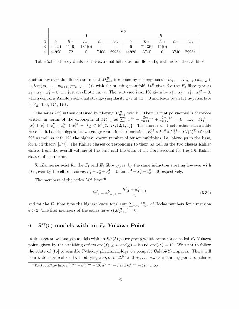
E6
A B
d χ h11 h21 h31 h22 χ h11 h21 h31 h22
3 −240 11(6) 131(0) − − 0 71(36) 71(0) − −4 44928 72 0 7408 29964 44928 3740 0 3740 29964
Table 5.3: F-theory duals for the extremal heterotic bundle configurations for the E6 fibre
duction law over the dimension in that MBn+1 is defined by the exponents m1, . . . ,mn+1, (mn+2 +
1), lcm(m1, . . . ,mn+1, (mn+2 + 1)) with the starting manifold MB1 given for the E8 fibre type as
x21 +x3
2 +x63 = 0, i.e. just an elliptic curve. The next case is an K3 given by x2
1 +x32 +x7
3 +x424 = 0,
which contains Arnold’s self-dual strange singularity E12 at x4 = 0 and leads to an K3 hypersurface
in P∆ [166, 175, 176].
The series MAn is then obtained by fibering MB
n−1 over P1. Their Fermat polynomial is therefore
written in terms of the exponents of MBn−1 as
∑ni1xmii + x
2mn+2
n+1 + x2mn+2
n+2 = 0. E.g. MA3 =
x21 + x3
2 + x73 + x84
4 + x845 = 0|x ∈ P4(42, 28, 12, 1, 1). The mirror of it sets other remarkable
records. It has the biggest known gauge group in six dimensions E178 ×F 16
4 ×G322 ×SU(2)32 of rank
296 as well as with 193 the highest known number of tensor multiplets, i.e. blow-ups in the base,
for a 6d theory [177]. The Kahler classes corresponding to them as well as the two classes Kahler
classes from the overall volume of the base and the class of the fibre account for the 491 Kahler
classes of the mirror.
Similar series exist for the E7 and E6 fibre types, by the same induction starting however with
M1 given by the elliptic curves x21 + x4
2 + x43 = 0 and x3
1 + x32 + x3
3 = 0 respectively.
The members of the series MBn have79
hB1,1 = hBn−1,1 =hA1,1 + hAn−1,1
2(5.30)
and for the E8 fibre type the highest know total sum∑
n,m hBn,m of Hodge numbers for dimension
d > 2. The first members of the series have χ(MB2n+1) = 0.
6 SU(5) models with an E8 Yukawa Point
In this section we analyze models with an SU(5) gauge group which contain a so called E8 Yukawa
point, given by the vanishing orders ord(f) ≥ 4, ord(g) = 5 and ord(∆) = 10. We want to follow
the route of [16] to sensible F-theory phenomenology on compact Calabi-Yau spaces. There will
be a wide class realized by modifying k, n,m or ∆(i) and n1, . . . , nm as a starting point to achieve
79For the K3 he have hB ver1,1 = hB hor
1,1 = 10, hA ver1,1 = 2 and hA hor
1,1 = 18, i.e. SA .
93

matter curves and an E8 point at codimension three in a compact case, in particular the examples
in Appendix A.1 for fourfolds with B3 = P1×P2 with an SU(5) gauge symmetry. Given the models
summarized in table A.1, there are two strategies either restricting a model with DG G ∈ E8 or
deforming a model with DE8 . We chose the first one, taking as departure a model with an SU(5)
singularity.
First we describe how a codimension 3 singularity with vanishing order of the coefficients to give
an E8 is obtained in the global construction described so far. Then we recall the SU(5) F-theory
GUT models using the notation which is present in the literature. Further, we describe the method
of the spectral cover used to parametrize the E8 singularities we plan to study. Then we come to
our focus which is the resolution of two models which posses a potentially E8 singularity: Case 1
and Case 2 in order to analyze the consequences of the non-applicability of Kodaira classification to
singularities with codimension higher than one [14]. For each of this cases we obtain fully resolved
spaces, and study the the codimension 2 and 3 loci and the gauge group charges of the different
matter curves.
6.1 A codimension three E8 point from the global construction
Consider the global toric construction employed for the tables in appendix A.1. It has polytope 1
in figure 1 and no twisting, giving B3 = P1 × P2. In this base it is possible to impose the existence
of certain codimension 3 singularities by fixing some moduli. We have search for a codimension 3
E8 singularity, such that the vanishing of the coefficients in the vicinity of the singular locus are
the ones in Table A.2.
Consider the variables of the base given by v, w, u1, u2, u3. Let us choose the 4-fold with a
codimension 1 singularity SU(5) at v = 0. This means that we obtain in (3.18) the following
dependence of the coefficients
a1 = f1(ui, w, cj) +O(v)g1(ui, w, v, cj), a2 = vf2(ui, w, cj) +O(v2)g2(ui, w, v, cj), (6.1)
a3 = v2f3(ui, w, cj) +O(v3)g3(ui, w, v, cj), a4 = v3f4(ui, w, cj) +O(v4)g4(ui, w, v, cj),
a6 = v5f6(ui, w, cj) +O(v5)g6(ui, w, v, cj).
We searched for a singularity in codimension-3 with the vanishing order for an E8 in the locus
v → t, u1 + u2 → t, u3 → t (parametrized via u1 → p+ t, u2 → −p), with t→ 0. This translates in
having
a1 = tl1(p, w, cj) +O(t2)m1(p, w, cj), a2 = t2l2(p, w, ci) +O(t3)m2(p, w, cj), (6.2)
a3 = t3l3(p, w, cj) +O(t4)m3(p, w, cj), a4 = t4l4(p, w, cj) +O(t5)m4(p, w, cj),
a6 = t5l6(p, w, cj) +O(t6)m6(p, w, cj).
This is achieved by looking at the pieces of the polynomial involving different vanishing order for
94

t. Let us look at the terms of order t0 in a1. The moduli that have to be fixed are the coefficients
of equation
(w2α3u31 + w2α5u
21u2 + w2α7u1u
22 + w2α10u
32)→ p3w2(−α3 + α5 − α7 + α10) , (6.3)
so we need to fix α3 → α5 − α7 + α10. For the coefficient a2 the terms of order t will be
(vw3β4u61 + vw3β8u
51u2 + vw3β12u
41u
22 + vw3β16u
31u
32 + (6.4)
vw3β20u21u
42 + vw3β24u1u
52 + vw3β28u
62)
→ tp6w3(β4 − β8 + β12 − β16 + β20 − β24 + β28) ,
so we need to fix β4 → β8− β12 + β16− β20 + β24− β28. For the coefficient a3 the terms of order t2
are given by
v2w4γ5u91 + v2w4γ10u
81u2 + v2w4γ15u
71u
22 + v2w4γ20u
61u
32 + v2w4γ25u
51u
42 + (6.5)
v2w4γ30u41u
52 + v2w4γ35u
31u
62 + v2w4γ40u
21u
72 + v2w4γ45u1u
82 + v2w4γ50u
92
→ t2p9w4(γ5 − γ10 + γ15 − γ20 + γ25 − γ30 + γ35 − γ40 + γ45 − γ50).
And the moduli should be fixed to make this last term vanish. For the coefficient a4 the following
terms contribute to the order t3 to give
v3w5(δ6u121 + δ12u
111 u2 + δ18u
101 u
22 + δ24u
91u
32 + δ30u
81u
42 + δ36u
71u
52 + (6.6)
δ42u61u
62 + δ48u
51u
72 + δ54u
41u
82 + δ60u
31u
92 + δ66u
21u
102 + δ72u1u
112 + δ78u
122 )
→ t3p12w5(δ6 − δ12 + δ18 − δ24 + δ30 − δ36 + δ42 − δ48 + δ54 − δ60 + δ66 − δ72 + δ78),
which has to vanish by setting the sum of the coefficients δ to zero. By fixing the moduli we have
arrived then to a 4-fold with a codimension 3 singularity which has the vanishing order of the so
called E8.
However in the given example we have fixed the moduli in excess. Let us argue that a more
satisfying solution with less relations constraining the moduli exists. We could impose the vanishing
of two coefficients at the required order, for example we can require f1 = f2 = 0 and search for
solutions in terms of u1 and u2 (setting u3 = 1, using the fact that (u1, u2, u3) ∈ P2), we obtain the
dependence u1(c1j , c2j) and u2(c1j , c2j). Having these solutions it will be sufficient to achieve the
required vanishing order to impose the following two relations among the moduli
f3(u1(c1j , c2j), u2(c1j , c2j), ω, c3j) = f4(u1(c1j , c2j), u2(c1j , c2j), ω, c4j) = 0. (6.7)
From the previous equations it is possible to eliminate the dependence on w, having two relations
which depend only on the moduli c1j , c2j , c3j and c4j . The vanishing order of the coefficients at
v = 0 and u1,2 fixed like u1,2(c1j , c2j) are given by 1, 2, 3, 4, 5, ensuring a so called E8 at codimension
3. General solutions of this kind can be found in the Calabi-Yau fourfolds we constructed.
95

Codimension 3 E8 singularities from the spectral cover
In this section we use the spectral cover construction, and in particular the breaking of the E8
coming from the decomposition in SU(5) × SU(5)⊥ by turning the values of the Higgs field ti to
be different from zero. When the ti → 0 for all i the E8 is recovered. Let us employ the relations
for the coefficients of the fibration in terms of the tis given in (6.30) and the parametrization for
the ti in terms of the variables p, q given in Case 1 from equation (7.1), one obtains that
a1 = β0(−4p3q2 − 4q4p− 10p2q3), a2 = β0(2p3q + 11p2q2 + 10pq3 + 4q4)w, (6.8)
a3 = β0(2p3 + 2p2q − 2pq2)w2, a4 = β0(−3p2 − 4pq − 5q2)w3.
a6 = β0w5.
At the codimension 3 locus determined by w = p = q = 0 the vanishing order of the coefficients
a1, a2, a3, a4, a6 is given by 5, 5, 5, 5, 5. This a case for the E8 singularity, different to the previously
discussed with the vanishing order 1,2,3,4,5. With the values given in (7) one can check that
ord(f) = 5 ≥ 4, ord(g) = 5 and ord(∆) = 10 which according to Table A.1 and [14, 35] constitutes
an E8.
We have explored various of the Calabi-Yau constructions presented and we found examples
where in a given patch, with a fine tuning of the moduli this type of singularity appears. One of
this cases is to have a model with an heterotic dual where B3 is constructed as a fibration of P1 over
P2 (polytope 1), with twist parameter m1 = −2 and other twists vanishing mk = 0. In this case
the coordinates of the P1 are denoted by v, w and the coordinates of the P2 by u1, u2, u3. Using
the notation u1 = p, u2 = q and setting many of the coefficients ckj to zero, one finds
a1 = v2(c11p3q2 + c12p
2q3 + c13pq4), a2 = v3u4
3(c21p3q + c22p
2q2 + c23pq3 + c24q
4)w, (6.9)
a3 = v4u83(c31p
3 + c32p2q + c33pq
2)w2, a4 = v5u123 (c41p
2 + c42pq + c43q2)w3,
a6 = v7u203 c61w
5.
We have omitted the higher order terms. For a patch in which v = u3 = 1 (6.9) coincides with (7).
One could explore other possibilities, for example with B3 = P1 → P2, twist m1 = −3 and mk = 0
this singularity kind can be obtained. However the polyhedra obtained from this tuning are not
reflexive, and we have lost the global description.
We have also explored the singularity type of Case 2 discussed in section 8. This case it is also
realized with B3 = P1 → P2, for m1 = −2 and other twists mk = 0. But the same difficulty of
the lost of reflexivity is present. We plan to consider in future work a detailed exploration of the
global models we have constructed to achieve a satisfactory global embedding of the codimension
3 E8 singularity and other singularities relevant to a 4d effective theory.
96

6.2 The SU(5) gauge group models
The equation for the elliptic fibration with coordinates x, y, z of a P2 bundle, in the patch z = 1,
and the base divisor w = 0 defining a codimension 1 A4 singularity is given by
− y2 + x3 + β0w5 + β2xw
3 + β3yw2 + β4x
2w + β5xy = 0, 80 (6.10)
in the Tate form (4.12), where the ai coefficients in (5.1) have been replaced by β6−iwi−1. Com-
paring to the Weierstrass form 3.1, we can identify the discriminant ∆ of the elliptic fibre and the
functions f and g.
∆ ≡− 16(−f3 + 27g2) = w5∆′,
f =1
48×3√
4(−β4
5 − 8β4β25w − 16β2
4w2 + 24β3β5w
2 + 48β2w3), (6.11)
g =−1
864(β6
5 + 12β4β45w + 48β2
4β25w
2 − 36β3β35w
2+
+ 64β34w
3 − 144β3β4β5w3 − 72β2β
25w
3 + 216β23w
4 − 288β2β4w4 + 864β0w
5),
with
∆′ = β5P + wβ5(8β4P + β5R) + w2(16β23β
34 + β5Q) + w3S + w4T + w5U, (6.12)
where P,R,Q, S, T and U are polynomials related to βi and w as
P = β23β4 − β2β3β5 + β0β
25 , R = 4β0β4β5 − β3
3 − β22β5, (6.13)
Q = −2(18β33β4 + 8β2β3β
24 − 15β2β
23β5 + 4β2
2β4β5 − 24β0β24β5 + 18β0β3β
25),
S = 27β43 − 72β2β
23β4 − 16β2
2β24 + 64β0β
34 + 96β2
2β3β5 − 144β0β3β4β5 − 72β0β2β25 ,
T = 8(8β3
2 + 27β0β23 − 36β0β2β4
), U = 432β2
0 .
So along GUT divisor w = 0, for general values of βis and as long as ∆′ remains non-vanishing,
the vanishing orders of ∆, f and g as we approach w → 0 are
ord(∆) = 5, ord(f) = 0, ord(g) = 0. (6.14)
and correspond to a singular curve of type I5, thus an A4 (or SU(5)) singularity.
Notice also that if we just fix all the parameters βi to zero except β0, we obtain an E8 singularity.
In fact, such an SU(5) model described by (6.10) can be seen as a higgsing of an E8 down to SU(5),
E8 → SU(5)× SU(5)⊥, (6.15)
80Here we change the notation with respect to the one in the equation of an E8 fibre (4.12). We do that in orderto ease the comparison with the literature [14, 15].
97

and the vevs for the Higgs are related to the sections βi. In the Type IIB picture, this can be
interpreted locally as a stack of five D7-branes separated by some distance (encoded by the vev of a
Higgs field), to other branes. As we move them close together the gauge group enhances. However,
from the pure perturbative description we cannot reproduce an E8-brane. If however we allow
ourselves to deepen in the strong coupling regime, we need to include (p,q)-7-branes, and open
strings that attach to 3 or more branes. These unusual open strings configurations can reproduce
an E8 algebra [178, 179].
In the following, we proceed to resolve the curve explicitly. First notice that (6.10) is singular
when w = x = y = 0. The βis depend on the coordinates on the base of the elliptic fibration B3.
They define holomorphic sections of the bundle O([6 − i]KB3 − [5 − i]SGUT), where KB3 is the
canonical bundle on the base B3. We perform the first blow up λ1 : [y, x, w], that is, introducing a
coordinate λ1 as
y = λ1y , x = λ1x , w = λ1w . (6.16)
together with the projective relations [y : x : w] . The defining equation (6.10) becomes
λ21(−y2 + λ1x
3 + β0λ31w
5 + β2λ21xw
3 + β3λ1yw2 + β4λ1x
2w + β5xy) = 0. (6.17)
The expression in brackets is the proper transform that defines Y4 (we reserve the symbol Y4 to the
fully resolved space), and the new homology class is given by
Y4 → Y4 + 2E1, (6.18)
where E1 = λ1. Y4 is still singular in y = x = λ1, and we blow up (we will reuse hatted coordinates
to denote all the intermediate blow ups, to avoid adding too many symbols and because we are
mainly interested in the original space and the final resolved one),
− y2 + λ2λ1x3 + β0λ2λ
31w
5 + β2λ2λ21xw
3 + β3λ1yw2 + β4λ2λ1x
2w + β5xy = 0, (6.19)
or, rearranging,
− y(y + β3λ1w
2 + β5x)
+ λ2λ1
(x3 + β0λ
21w
5 + β2λ1xw3 + β4x
2w)
= 0. (6.20)
The space is smooth in general points of the GUT divisor, but it acquires further singularities
when we approach particular values for the βis, corresponding to subregions on SGUT. The reso-
lution of these singularity enhancements were performed via small resolutions in the work of Esole
and Yau [14] and reviewed in a series of other papers [180, 181, 15]. These enhancements lead to
fiber structures that reproduce the fundamental and the antisymmetric representations 5 and 10
of the SU(5) gauge group, the two representations required to construct matter in realistic SU(5)
models. Furthermore, there are points on the base (codimension three) where the singularities en-
hance even further, corresponding to places where matter curves intersect. These points reproduce
98

the couplings 10 10 5 and 10 5 5, required to reproduce the Yukawa couplings between quarks and
the Higgs field.
In particular, at the point on the base defined by w = β4 = β5 = 0, when these coordinates
are treated as non-factorizable holomorphic variables, the explicit resolution does not give for the
blown-up P1s the geometric structure corresponding to the Dynkin diagram of an E6 group, as
expected from the counting of the vanishing order as in table A.1. Further analysis [15] showed
that although the resolution does not reproduce the exact diagram that would be naively expected
from the Tate’s algorithm, it still reproduces the 10 10 5 coupling, necessary to give mass to the
top quark in an SU(5) GUTs, the main reason for why one considers E6 enhancements in the first
place.
However, Esole-Yau resolution [14] does not contemplate further singularities, that can arise
in particular regions on the moduli space of the base where the parameters βi factorize. Such
possibility of factorization was studied in other contexts for example in [181, 182].
We also propose a factorization to reproduce a codimension 3 (a point on the base) enhancement
to an E8 singularity. Our construction of such splitting follows from the established connections
between F-theory and heterotic string theory, where the coefficients βi are related to the higgsings
used to break E8 down to SU(5), as
E8 −→ SU(5)× SU(5)⊥. (6.21)
We will briefly review how are the coefficients in the elliptic fiber related to the Higgs vevs in the
next section, following [183, 184].
6.3 The βi Coefficients from the Spectral Cover
The rough idea of the spectral cover construction is to incorporate in a geometrical description the
higgsing of a gauge group. Our starting point is the E8 group, that we break down to an SU(5),
E8 → SU(5)× SU(5)⊥ → SU(5)× U(1)4. (6.22)
There is a Higgs field responsible for the breaking, which can be locally described as a section of
the canonical bundle over the SU(5) divisor S with values on the adjoint of E8,
KS ⊗Adj(E8). (6.23)
In standard geometrical engineering, the gauge groups are identified with singularities as the stan-
dard ADE classification, obtained as a blow-down of the resolved geometry. They are then broken
to smaller subgroups by giving non-vanishing volume to some P1’s. This corresponds to giving a
vev to the Cartans of SU(5)⊥. Thus, being a Cartan root, the Higgs field we are interested in
obeys [Φ,Φ†] = 0. These solutions are also relevant since they usually leave N = 1 supersymmetry
unbroken.
99

We next want to describe the Higgs field in terms of its eigenvalues and eigenvectors, that is,
its spectral data. We introduce a section s of the canonical bundle over S, KS , and we can write
the eigenvalue equation
det(sI − Φ) = 0. (6.24)
Since we restrict to the Higgs field that leaves the SU(5) but breaks SU(5)⊥, we can expand (6.24)
in the 5 eigenvalues ti for the fundamental representation of SU(5)⊥ as∏i
(s− ti) = 0. (6.25)
Expanding, we find
β0s5 + β2s
3 + β3s2 + β4s+ β5 = 0. (6.26)
The β1 is not present since β1 = t1 + ... + t5 = 0, from the tracelessness condition of the roots in
SU(5). Although it is not yet clear, the βis in (6.26) are the same as the elliptic fiber equation
in the Tate form, when in the vicinity of the GUT divisor. To see that, we first define the “Tate
divisor” [15], as the equation
CTate : β0w5 + β2xw
3 + β3yw2 + β4x
2w + β5xy = 0. (6.27)
The equation for the elliptic fiber (6.10),
− y2 + x3 +(β0w
5 + β2xw3 + β3yw
2 + β4x2w + β5xy
)= 0, (6.28)
when restricted to the Tate divisor implies y2
x3 = 1. Also we can define the holomorphic section
u = y/x on the Tate divisor. This allows us to write the Tate divisor as
CTate : β0w5 + β2w
3u2 + β3w2u3 + β4wu
4 + β5u5 = 0. (6.29)
We then restrict to the vicinity of w → 0 and close to the singularity on the elliptic fiber y → 0,
x→ 0. This in turn implies u→ 0. We consider the section s = w/u in (6.29), to arrive precisely
at the spectral curve (6.26). The coefficients βi are given in terms of the eigenvalues ti as
β1 = −β0
∑i
ti = 0, β2 = β0
∑i 6=j
titj , (6.30)
β3 = −β0
∑i 6=j 6=k
titjtk, β4 = β0
∑i 6=j 6=k 6=l
titjtktl, β5 = −β0t1t2t3t4t5.
Recall also that the first enhancements that we encounter in the SU(5) model happens when
∆′ in ∆ = w5∆′ has a first order zero. This corresponds to the vanishing of
β5 = −β0t1t2t3t4t5 , or (6.31)
P5 = −β30
∏i 6=j
(−ti − tj) = β23β4 − β2β3β5 + β0β
25 .
100

The expansion of the f, g and ∆ in terms of the variables on the singularity w and ti is given
by
∆ = −432β20w
10 + . . . f = β0
∑i 6=j
titjw3 + . . . , g = β0w
5 + . . . , (6.32)
where the dots indicate higher order terms in w. As we want an enhancement to an E8, it follows
from the Kodaira classification A.1 that we should have
ord(f) ≥ 4 , ord(g) = 5 , ord(∆) = 10 . (6.33)
In order to achieve ord(f) ≥ 4 we require every term titj to vanish, that in turn imposes at
least 4 of the tis to be zero. But from the tracelessness condition, it implies that all should be zero.
We could have advanced this, since the tis are related to higgsings of the underlying E8 group, so
setting all tis to zero would un-break the E8.
Since we want to describe this enhancement as a codimension 3 locus, we introduce sections p
and q, that will be normal sections to curves on the SU(5) divisor. We could interpret this as the
normal sections of divisors on the base B3, but as we will argue later, having started from the Tate
model does not allow this interpretation. Looking at β2 relation with β0 this means that∑
i 6=j titj
must be a section of the K−2B3⊗ L2
SU(5).
We impose now that the ti’s can be written as
ti = tpi p+ tqi q. (6.34)
The tpi and tqi could also be sections of some bundle on the base, but for simplicity of the model
we consider them to be constant integer numbers. This implies that p and q are sections of
K−1B3⊗ LSU(5), and could be homologically equivalent to each other. The tracelessness condition
β1 = 0 implies
p(tp1 + tp2 + tp3 + tp4 + tp5) + q(tq1 + tq2 + tq3 + tq4 + tq5) = 0.
We also want no trivial solution to (6.31), thus ti 6= 0 and ti + tj 6= 0. In the next sections we
will consider two different cases that satisfy the above requirements and reproduce a point of E8
singularity.
7 Case 1: E8 model with the 5 and the 10 matter representations
One choice that satisfies all the requirements for an E8 point is
t1 = p, t2 = q, t3 = p+ 2q, t4 = −2p− q, t5 = −2q. (7.1)
101
The βis after the replacements (6.34) become
β2 = −β0(3p2 + 4pq + 5q2), β3 = 2β0p(p2 + pq − q2),
β4 = β0q(2p3 + 11p2q + 10pq2 + 4q3), β5 = −2β0pq
2(2p+ q)(p+ 2q).
It is also convenient, for reference, to write the polynomials P and R,
P =4β30p
2(p− 2q)(p− q)q(p+ q)3(p+ 3q)(2p+ 3q), (7.2)
R =− 2β30p(p+ q)2(4p6 + 4p5q − 30p4q2 − 41p3q3 + 10p2q4 − 9pq5 − 18q6).
Replacing the values for the βi’s, equation (7.2),
y2 − 2β0pq2(2p+ q)(p+ 2q)xyw + 2β0p
(p2 + pq − q2)
)yw2 + x3 + β0w
5+ (7.3)
−β0
(3p2 + 4pq + 5q2
)xw3 + 2β0q(2p
3 + 11p2q + 10pq2 + 4q3)x2w = 0.
We next calculate explicitly f , g and ∆ as depending on w, p and q. There will be codimension
two and three loci on the base where the vanishing order of these functions will increase. If we
extrapolate the result of the Kodaira classification (table A.1) to codimension higher than one,
we can extract the information on the “expected” gauge group over each locus. Away from the
enhancement loci and close to w = 0, we find
f = −1
3b04p4q8(2p+ q)4(p+ 2q)4 +O(w) ,
g =2
27b06p6q12(2p+ q)6(p+ 2q)6 +O(w) , (7.4)
∆ = −64(b07p6q9(p+ q)3(2p2 + 5pq + 2q2)4(2p4 + 3p3q − 14p2q2 − 9pq3 + 18q4))w5 +O(w6),
and therefore ord(∆) = 5 and ord(f) = ord(g) = 0. Over the codimension 2 locus p = 0 together
with w = 0, we obtain ord(∆) = 8, ord(f) = 2 and ord(g) = 3, the vanishing degrees for an SO(12)
singularity, while the curve q = 0 corresponds to an E6 singularity. Notice that in general (non-
factorized βis) SO(12) and E6 singularities appear only at codimension 3, reproducing the 1055
and 10105 couplings, respectively. In the next sections we will discuss what matter representation
can be obtained after we resolve these singularities.
We can identify other enhancement loci that we summarize in table 7.1. We will call the
w = q = 0 locus the E6 matter curve, even if the explicit resolution lead to something different
from an E6. Similar notation will apply to the other codimension two loci.
At the point p = q = w = 0 in which we expect by construction to get a E8 singularity, one
can check that we get exactly ord(∆) = 10, ord(f) = 5 and ord(g) = 5, the expected for a E8
singularity. Similarly, we call this codimension three locus the E8 Yukawa point.
102

Locus (in w = 0) Codim ord (∆/f/g) Sing. type
p = 0
2
8/2/3 SO(12)q = 0 8/3/4 E6
p+ q = 0 7/0/0 SU(7)p− 2q = 0
6/0/0 SU(6)p− q = 0p+ 3q = 02p+ 3q = 02p+ q = 0
7/2/3 SO(10)p+ 2q = 0
p = q = 0 3 10/5/5 E8
Table 7.1: Codimension 2 and 3 enhancements for the particular model (6.34).
7.1 Resolution
After we replace the values of the βi’s for our chosen factorization (7.1) the expression for the
elliptic curve becomes
y2z − 2β0p(p2 + pq − q2)w2yz2 + 2β0pq
2(2p+ q)(p+ 2q)xyz − x3 − β0w5z3
+β0(3p2 + 4pq + 5q2)w3z2x− β0q(2p3 + 11p2q + 10pq2 + 4q3)x2wz = 0 .
After the two first blow ups, we again have a binomial variety of the form encountered before,
zys+ λ1λ2(. . .) = 0, (7.5)
with s = −y − 2β0pq2(2p + q)(p + 2q)x + 2β0p(p
2 + pq − q2)w2z. We resolve the singularities by
performing the small resolutions δ1 : [y, λ1] and δ2 : [y, λ2],
0 = yz(β0pq
2(4p2 + 10pq + 4q2)x+ δ1δ2y + δ1λ1β0p(−2p2 − 2pq + 2q2)w2z)
+λ1λ2
(−δ2λ2x
3 − β0q(2p3 + 11p2q + 10pq2 + 4q3)wx2z (7.6)
−β0δ1λ1(−3p2 − 4pq − 5q2)w3xz2 − β0δ21λ
21w
5z3),
with the projective relations
[δ2δ1λ2y : δ2λ2x : w], [δ2δ1y : x : δ1λ1], [δ2y : λ1], [y : λ2]. (7.7)
The coordinates describe sections of bundles as shown in table B.1, in Appendix B.
At this point, as in Esole-Yau resolution [14] we would have the fully resolved space. The
enhancements studied do not worsen the singularities, but only split the already existing curves.
In our particular construction, however, there are further singularities to be resolved. The reason
for this is that in our model the βi’s split in a product of the sections p and q, thus enhancing the
vanishing order of the previously smooth terms.
103

All the further singularities are located on top of q = 0. After resolving for generic points in p,
there are still some singularities on the point q = p = 0. We can resolve the singularities by many
different ways. We choose the particular resolution
χ1 : [q, λ2, δ1], χ2 : [χ1, δ1], χ3 : [χ2, p, δ2], χ4 : [χ3, δ2], χ5 : [χ4, δ2], (7.8)
resulting in the following expression for the resolved fourfold,(−δ2λ2χ1x
3 + b0qχ1χ23χ4(−2p3 − 11p2qχ1χ2 − 10pq2χ2
1χ22 − 4q3χ3
1χ32)wx2z +
−β0χ1χ2χ23χ4(−3p2 − 4pqχ1χ2 − 5q2χ2
1χ22)δ1λ1w
3xz2 − β0δ21λ
21χ
21χ
32χ
23χ4w
5z3)λ1λ2 + (7.9)
+(β0pq
2χ1χ23(4p2 + 10pqχ1χ2 + 4q2χ2
1χ22)χ4x+
+2β0pχ23χ4(−p2 − pqχ1χ2 + q2χ2
1χ22)δ1λ1w
2z + δ1δ2y)yz = 0
Notice that some of the blow-ups were performed by introducing P2s in the ambient space, while
in the Esole-Yau small resolutions we had only P1s. As a consequence, we are in fact introducing
a new (three-dimensional) divisor on the fourfold, but localized along codimension 2 on the base
(the matter curve). That is, the new fiber will have to have dimension higher than one. Up to now,
the effect of the resolutions was only to modify the one-dimensional fiber of the fourfold, replacing
the singular points by one dimensional curves. In the resolution we will perform now, we then also
modify the base of the fibration, introducing new submanifolds along the enhancement loci.
The difference here to the previous case where we only needed small resolutions lies on the
fact that, in the brane picture, the collisions that lead to SU(6) and SO(10) matter curves come
from collision of the SU(5)-brane with an U(1) seven-brane or an O7-plane. Both correspond to
a non-singular degeneration of the fiber, and therefore a resolution is not needed. In this case,
however, the collision inducing an E6 enhancement can be understood as
E6 → SU(5)× SU(3), (7.10)
and thus the colliding brane would carry with it a singularity from the F-theory perspective. Our
local construction however does not allow us to see the colliding brane outside the SU(5) locus
w = 0.
The coordinates in (7.9) obey the list of projective relations
104

δ21δ
32λ1λ
22χ
41χ
62χ
93χ
124 χ
155 y : δ2
2λ1λ22χ1χ2χ
23χ
34χ
45x : z 6= 0 : 0 : 0
δ1δ22λ2χ
21χ
32χ
53χ
74χ
95y : δ2λ2χ1χ2χ
23χ
34χ
45x : w 6= 0 : 0 : 0,
δ1δ2χ1χ22χ
33χ
44χ
55y : x : δ1λ1χ1χ
22χ
23χ
24χ
25 6= 0 : 0 : 0, (7.11)
δ2χ3χ24χ
35y : λ1 6= 0 : 0, y : λ2χ1χ2χ3χ4χ5 6= 0 : 0,
q : λ2 : δ1χ2χ3χ4χ5 6= 0 : 0 : 0,
χ1 : δ1 6= 0 : 0, χ2 : p : δ2χ4χ25 6= 0 : 0 : 0,
χ3 : δ2χ5 6= 0 : 0 : χ4 : δ2 6= 0 : 0;
and are sections of the bundles from table B.1.
The class of the new fourfold Y4 is given by
[Y4] = 3σ + 6c1 − 2E1 − 2E2 − E3 − E4 − E5 − E6 − E7 − E8 − E9. (7.12)
7.2 Codimension 1 - The GUT Divisor
At codimension one, when we restrict ourselves to χ3χ4χ5p 6= 0, χ1χ2χ3χ4χ5q 6= 0, we can simply
blow down the five last blow-ups since they all sit along χ3χ4χ5p = 0 or χ1χ2χ3χ4χ5q = 0. Blowing
down, we simply return to our space after the two small resolutions, (7.6). Working in the partially
or the full blown-up space the singularity of the fiber is resolved and we get five curves, ordered as
the picture below,
HHH
A B C D
X
where the curves are given by the restriction of the ambient divisors
A : δ1 = 0, B : δ2 = 0, C : λ2 = 0, D : λ1 = 0 , (7.13)
to the fourfold Y4. The defining equations are exhibited in appendix B. One can calculate the
intersections among the divisors restricted to the fiber in the same way as was done in [15, 185],
and we get precisely the Cartan matrix (times −1) for an SU(5) group,
A B C D XA
-2 1 0 0 11 -2 1 0 00 1 -2 1 00 0 1 -2 1
1 0 0 1 -2
BCDX
105

7.3 Codimension 2
Now we look at the codimension 2 loci, where the matter representations appear.
7.3.1 10 Matter Curve
We start with the locus p + 2q = 0 from the singular fourfold, that from the vanishing degree
corresponded to an SO(10) enhancement, and from group-theoretical arguments to a matter 10
representation. After the complete resolution of the fourfold, the locus is defined by p+ 2qχ1χ2 ≡p0 + 2q0 = 0, and the expression for the fourfold reduces to
0 = −y2zδ1δ2 + x3δ2λ1λ22χ1 + β0w
5z3δ21λ
31λ2χ
21χ
32χ
23χ4 − 4β0q
3w2yz2δ1λ1χ31χ
32χ
23χ4 (7.14)
−9β0q2w3xz2δ1λ
21λ2χ
31χ
32χ
23χ4 + 12β0q
4wx2zλ1λ2χ41χ
32χ
23χ4 ,
with the projective relations (7.11). As in [14, 15], the divisors living in codimension 1 now rearrange
themselves in a different way, by splitting into new curves or merging with one another. Namely,
the restriction to the fourfold of the divisor δ1 = 0 at the p− 2qχ1χ2 = 0 locus becomes
λ1λ2χ1x2(δ2λ2x+ 12β0q
4χ31χ
32χ
23χ4wz) = 0, (7.15)
that is factorizable in three different curves (obeying the projective relations (7.11))
Dp−2q0 : λ1 = 0, A1p−2q0 : λ2 = 0, A2p−2q0 : δ2λ2x+ 12β0q4χ3
1χ32χ
23χ4wz = 0. (7.16)
A similar splitting happens for the divisor λ2 = 0, as in the fourfold
δ1yz(δ2y + 4β0λ1q3χ3
1χ32χ
23χ4w
2z) = 0, (7.17)
that factors in
A1p−2q0 : δ1 = 0 and Cp−2q0 : δ2y + 4β0λ1q3χ3
1χ32χ
23χ4w
2z = 0. (7.18)
We then calculate the intersection of these curves with the Cartan divisors (7.13) to get the charges
of each curve under the Cartan roots, obtaining (details in appendix C)
One can check that the weights obey the charge conservation
A = A1p−2q0 +A2p−2q0 +Dp−2q0,
C = Cp−2q0 +A1p−2q0,
the curves in table 7.2 reproduce a complete representation of the matter 10, and they distribute
themselves as the Dynkin diagram for the SO(10) group.
106

Curve Charges Weights
A1p−2q0 (-1,1,-1,1,0) µ10 − α1 − α2 − α3
A2p−2q0 (-1,0,0,1,0) −µ10 + α2 + α3 + α4
Bp−2q0 (1,-2,1,0,0) −α2
Cp−2q0 (1,0,-1,0,0) −µ10 + α1 + α2
Dp−2q0 (0,0,1, -2, 1) −α4
Xp−2q0 (1,0,0,1,-2) −α0
Table 7.2: Curves over the locus p− 2qχ1χ2 ≡ p− 2q0 = 0 with their corresponding charges. Thedefining equations are in table B.10.
7.3.2 Matter 5
The matter 5 representation is expected to appear at the SU(6) enhancement locus, where P = 0.
In our model, there are many loci that describe this enhancement. We will focus on p− q = 0. An
analogous calculation follows for the other matter 5 loci, but with different numerical factors.
At this locus, the curve specified by δ2 = 0 becomes reducible. Namely, the defining equation
for this curve at the fourfold becomes (with χi = 1)
− β0z(−9q2x+ δ1λ1w
2z) (−3λ1λ2q
2wx+ 2q3y + δ1λ21λ2w
3z), (7.19)
that is factorizable in two curves,
B1p−q0 : δ2 = −9q2x+ δ1λ1w2z = 0 and B2p−q0 : δ2 = −3λ1λ2q
2wx+ 2q3y + δ1λ21λ2w
3z = 0
(7.20)
It is then straightforward to calculate the weights for the new curves.
Curve Charges Weights
A1p−q0 (-2,1,0,0,1) −α1
Bp−q0 (1,-1,0,0,0) −µ5 + α2
Bp−q0 (0,-1,1,0,0) −µ5 + α2
Cp−q0 (0,1,-2,1,0) −α3
Dp−q0 (0,0,1, -2, 1) −α4
Xp−q0 (1,0,0,1,-2) −α5
Table 7.3: Curves over p− q0 = 0. Defining equations in table B.3..
Again, the splitting reproduces a full matter 5 representation, and arrange themselves as the
Dynkin diagram for the SU(6) group.
107

7.3.3 The p = 0 and the q = 0 loci
We now describe two interesting codimension 2 loci that do not appear in previous works. When
p = 0, the curves split as
A : δ1p→0−−−→ A1p : δ2λ2x+ 4β0q
4χ31χ
32χ
23χ4wz = 0, A2p : λ2 = 0, A3p : λ1 = 0 ,
B : δ2p→0−−−→ B1p : λ2 = 0, B2Ap : −q2χ1x+ δ1λ1w
2z = 0, B2Bp : −4q2χ1x+ δ1λ1w2z = 0,
C : λ2p→0−−−→ A3p : δ1 = 0, B1p : δ2 = 0, (7.21)
and rearrange as the SO(12) Dynkin diagram. The calculation of the intersections between the
curves in the p = 0 locus with the Cartan divisors again give the weights of each curve under the
SU(5) group,
Curve Charges Weights
A1p (-1,1,-1,1,0) µ10 − α1 − α2 − α3
A2p (-1,0,0,1,0) −µ10 + α2 + α3 + α4
B1p (1,0,-1,0,0) −µ10 + α1 + α2
B2Ap (0,-1,1,0,0) µ5 − α1 − α2
B2Bp (0,-1,1,0,0) µ5 − α1 − α2
Dp (0,0,1,-2, 1) −α4
Xp (1,0,0,1,-2) −α0
Interestingly, this set of curves reproduces a full representation 5+10. To check that, notice first
that B2Ap +B1p = (1,−1, 0, 0, 0) = −µ5 +α1. One can then reconstruct the full representation
by appropriate combinations of the curves above.
Over the q0 = 0 locus we have to be more careful. The locus is described after the blow-up by
qχ1χ2 = 0. Thus, one has to see the behaviour of the Cartan roots as we approach q → 0, χ1 → 0
and χ2 → 0.
The roots as we take q → 0 are
A : δ1q→0−−−→ Aq : δ2 = 0, Dq : λ1 = 0,
B : δ2q→0−−−→ Aq : δ1 = 0, Bq : 3λ1λ2p
2χ1χ2wx+ 2p3y − δ1λ21λ2χ
21χ
32w
3z = 0,
C : λ2q→0−−−→ Cq : δ2y + 2β0λ1p
3χ23χ4w
2z = 0,
D : λ1q→0−−−→ Dq : δ1 = 0.
When we calculate the charges under the SU(5) roots, only the above curves will have non-
vanishing contributions, while all the curves appearing as we take χ1 → 0 or χ2 → 0 have zero
charge81. Thus, the only contributing curves are given in the table below:
81The calculation of the intersections give terms like D1S2Eiσ2, that vanish since D1, S2 and σ are pullbacks from
the blow-down to the blow-up space.
108

Curve Charges Weights
Aq (0,-1,1,0,0) µ5 − α1 − α2
Bq (1,-1,0,0,0) −µ5 + α1
Cq (1,0,-1,0,0) −µ10 + α1 + α2
Dq (0,0,1,-2,1) α4
Xq (1,0,0,1,-2) α0
Table 7.4: Curves of non-vanishing charges on the q = 0 locus. Defining equations in B.6
There is a breaking of the charge conservation, as the daughter curves do not reproduce the
weights of the original (codimension 1) ones. Namely, the difference can be solved by a single curve
M of charges (−1, 1,−1, 1),
A → 2M +Aq +Dq
(−2, 1, 0, 0, 1) = (−2, 2,−2, 2, 0) + (0,−1, 1, 0, 0) + (0, 0, 1,−2, 1),
C → M + Cq
(0, 1,−2, 1, 0) = (−1, 1,−1, 1, 0) + (1, 0,−1, 0, 0).
The curve M has weight in the 10 representation, namely (µ10 − α1 − α2 − α3).
The curves now do not form a recognizable Dynkin diagram. In fact, if we consider only the
curves from table 7.4 the fiber structure is split as the picture 3a below. If however we include the
curves not charged under the SU(5), we get a connected set of curves, as picture 3b.
Dq Cq Aq Bq Xq
(a) The curves from table 7.4 (b) Including the uncharged curves
Figure 3: Curves on the q0 = 0 locus.
7.4 Codimension 3
As we move to the point p0 = q0 = 0, again we have more than one vanishing section in the blow-up
space, since p0 = q0 = 0 → pχ3χ4χ5 = qχ1χ2χ3χ4χ5 = 0. But just like the q0 = 0 locus, only
the restriction p = q = 0 gives non-vanishing charge subspaces under the SU(5). These spaces are
given in the table 7.5 below, while the defining equations are given in the appendix B.
We took care not to call these spaces “curves” since unlike the ones appearing in codimension
2, these are not P1s inside the fourfold fiber. This is a consequence of the fact that by blowing up
we introduced new exceptional divisors over the point of the base p0 = q0. The fiber then is not
one-complex-dimensional.
109

Curve Equations Charges Weights
AE8 δ1 = δ2 = 0 (0,-1,1,0,0) µ5 − α1 − α2
CE8 δ2 = λ2 = 0 (1,0,-1,0,0) −µ10 + α1 + α2
DE8 λ1 = δ1 = 0 (0,0,1,-2,1) α4
XE8 w = Y4|w=0 = 0 (1,0,0,1,-2) α0
Table 7.5: Curves of non-vanishing charges on the p0 = q0 = 0 point. Equations in B.7.
In the next section we will explore another resolution in which we have a better control on these
higher dimensional subspaces appearing after the blow-up.
8 Case 2: E8 model with p0 and q0 symmetric
We now choose for the higgsings (6.34)
t1 = p, t2 = q, t3 = p+ q, t4 = −2q, t5 = −2p. (8.1)
This particular selection is symmetric under the exchange p ↔ q. Physically, this means the
matter curves represented by p = w = 0 and q = w = 0 could be exchanged. The role of exchange
symmetries for the curves in phenomenological F-theory models was explored for example in [16].
The βis after the replacements (8.1) become
β2 = −β0(3p2 + pq + 3q2), β3 = β0(p+ q)(2p2 − 3pq + 2q2), (8.2)
β4 = 2β0pq(p2 + 4pq + q2), β5 = −4β0p
2q2(p+ q).
It is also convenient, for reference, to write the polynomials P and R,
P =2β30p(p− 2q)(p− q)2(2p− q)q(p+ q)2(2p+ q)(p+ 2q), (8.3)
R =− β30(p− q)2(p+ q)(8p6 − 4p5q − 38p4q2 − 43p3q3 − 38p2q4 − 4pq5 + 8q6).
Replacing the values for the βi’s, equation (8.2),
− y2z − 4β0p2q2(p+ q)xyz + β0
[2(p3 + q3)− pq(p+ q)
]yw2z2 + x3 + β0w
5z3+ (8.4)
+β0
[−3(p2 + q2)− pq
]xw3z2 + 2β0pq(p
2 + q2 + 4pq)x2wz = 0.
We again calculate explicitly f , g and ∆ with respect to w, p and q. On the codimension 2
locus p = 0 together with w = 0, we get
∆ = −432q12w8 + . . . ,
f = −3q2w3 + . . . , (8.5)
g = q6w4 + . . . ,
110

where the . . . are terms of higher vanishing order. Therefore ord(∆) = 8, ord(f) = 3 and ord(g) = 4,
the vanishing degrees for a E6 singularity. There are also other codimension 2 enhancements
appearing in p± q = 0, p± 2q = 0 and 2p± q = 0, that we summarize in table 8.1. We will call the
w0 = p0 = 0 locus the E6 matter curve, even if the explicit resolution leads to something different
from an E6. Similar notation will apply to the other codimension two loci.
At the point p = q = w = 0 in which we expect by construction to get an E8 singularity,
∆ = −432w10 + . . . ,
f = −3p2w3 − pqw3 − 3q2w3 + . . . , (8.6)
g = w5 + . . . ,
Thus ord(∆) = 10, ord(f) = 5 and ord(g) = 5, the expected for a E8 singularity. Similarly, we call
this codimension three locus the E8 Yukawa point.
Curve (in w = 0) Codim ord (∆/f/g) Sing. type
p = 0, q = 0
2
8/3/4 E6
p+ q = 0 8/2/3 SO(12)p− q = 0 7/0/0 SU(7)
p± 2q = 0, q ± 2p = 0 6/0/0 SU(6)
p = q = 0 3 10/5/5 E8
Table 8.1: Codimension 2 and 3 enhancements for the particular model (8.1).
8.1 Resolution
Replacing the expressions for the βis for the case (8.2) into the expression for the elliptic fibration
4.12 and performing the two blow-ups λ1 : [y, x, w] and λ2 : [y, x, λ1] we get,
zy(−y − 4β0p2q2(p+ q)x+ β0
[2(p3 + q3)− pq(p+ q)
]λ1zw
2)+ (8.7)
+λ2λ1(λ2x3 + λ2
1w5z3β0 + β0
[−3(p2 + q2)− pq
]λ1w
3xz2 + 2β0pq(p2 + q2 + 4pq)x2wz) = 0 .
We have a binomial variety of the form encountered in [14, 15],
zys+ λ1λ2(. . .) = 0, (8.8)
with s = −y−4β0p2q2(p+q)x+β0
[2(p3 + q3)− pq(p+ q)
]λ1w
2z. We perform the small resolutions
δ1 : [y, λ1] and δ2 : [s, λ2],0 = zys+ λ2λ1(δ2λ2x
3 + δ21λ
21w
5z3 + β0
[−3(p2 + q2)− pq
]δ1λ1w
2x+ 2β0pq(p2 + q2 + 4pq)x2wz)
0 = δ2s+ δ1y + 4β0p2q2(p+ q)x− β0
[2(p3 + q3)− pq(p+ q)
]δ1λ1w
2z ,
(8.9)
111

with the projective relations
[δ2δ1λ2y : δ2λ2x : w], [δ1y : x : δ1λ1], [y : λ1], [s : λ2]. (8.10)
The coordinates describe sections of the bundles as follows
x σ + 2c1 − E1 − E2
y σ + 3c1 − E1 − E2 − E3
s σ + 3c1 − E1 − E2 − E4
w S2 − E1
z σλ1 E1 − E3
λ2 E2 − E4
δ1 E3
δ2 E4
p, q S2 − c1
β0 6c1 − 5S2
Table 8.2: Coordinates and their respective bundles.
At this point, as in Esole-Yau resolution [14] we would have the fully resolved space. The
enhancements studied there do not worsen the singularities, but only split the already existing
curves. In our particular construction, however, there are further singularities to be resolved. The
reason for this is that in our model the βi’s split in a product of the sections p and q, enhancing
the vanishing order of the previously smooth terms.
We now proceed to resolve the additional singularities. First, we rearrange equation (8.1) as 820 = ys+ λ2λ1(δ2λ2x
3 + δ21λ
21w
5 + β0
[−3(p2 + q2)− pq
]δ1λ1w
2x+ 2β0pq(p2 + q2 + 4pq)x2w) ,
0 = δ2s+ δ1
(y − β0
[2(p3 + q3)− pq(p+ q)
]λ1w
2)
+ 4β0p2q2(p+ q)x .
We note that all the singularities of the second equation arise when δ2 = δ1 = s = (...) = p = 0.
or δ2 = δ1 = s = (...) = q = 0. Similarly as was done to resolve the SU(5), we introduce an
auxiliary equation t = y −[2(p3 + q3)− pq(p+ q)
]λ1w
2, and we work with the system of three
equations,0 = ys+ λ2λ1(δ2λ2x
3 + δ21λ
21w
5 + β0
[−3(p2 + q2)− pq
]δ1λ1w
2x+ 2β0pq(p2 + q2 + 4pq)x2w) ,
0 = δ2s+ δ1t+ 4β0p2q2(p+ q)x ,
0 = −t+ y − β0
[2(p3 + q3)− pq(p+ q)
]λ1w
2 .
(8.11)
It is now straightforward to resolve this system of equations. First we resolve the singularity at
q = s = t = δ1 = δ2 = 0 in the second equation, by performing the blow up χ1 : [s, t, q], that is
s→ χ1s, t→ χ1t, q → χ1q, with the projective relation [s : t : q]. (8.12)
82We set z = 1, as we are concerned with singularities in the patch z 6= 0. We reintroduce it back at the end.
112

Notice that this was a P2 blow up, not a small resolution as was done to resolve the curves
and Yukawa enhancements in the previous section. As a consequence, we are in fact introducing
a new (three-dimensional) divisor on the fourfold, but localized along codimension 2 on the base
(the matter curve). That is, the new fiber will have to have dimension higher than one. Up to now,
the effect of the resolutions was only to modify the one-dimensional fiber of the fourfold, replacing
the singular points by one dimensional curves. In the resolution we will perform now, we then also
modify the base of the fibration, introducing new submanifolds along the enhancement loci.
The difference here to the previous case where we only needed small resolutions lies on the
fact that, in the brane picture, the collisions that lead to SU(6) and SO(10) matter curves come
from collision of the SU(5)-brane with an U(1) seven-brane or an O7-plane. Both correspond to
a non-singular degeneration of the fiber, and therefore a resolution is not needed. In this case,
however, the collision inducing an E6 enhancement can be understood as
E6 → SU(5)× SU(3), (8.13)
and thus the colliding brane would carry with it a singularity from the F-theory perspective. Our
local construction however does not allow us to see the colliding brane outside the SU(5) locus
w = 0.
One should also keep in mind that there is a large number of possibilities for the blow-ups, that
might lead to different final resolved manifolds. Here we perform one of many choices, that leads
to a resolved space in few steps. There is however no possibility to resolve this singular space only
via small resolutions. To fully resolve the space, we then choose to perform other three blow ups,
in the following order,
χ2 : [s, t, χ1], π1 : [s, t, p], π2 : [s, t, π1], (8.14)
thus introducing four new divisors to the ambient fivefold given by π1 = 0, π2 = 0, χ1 = 0and χ2 = 0.
The defining equations for the elliptic fiber consists now on the triple intersection (with z
reintroduced)0 = π1π
22χ1χ
22zsy + λ1λ2(−2β0pπ1π2qχ1χ2(p2π2
1π22 + 4pπ1π2qχ1χ2 + q2χ2
1χ22)x2wz−
−β0δ21λ
21w
5z3 + β0δ1λ1(3p2π21π
22 + pπ1π2qχ1χ2 + 3q2χ2
1χ22)w3xz2 − δ2λ2x
3) ,
0 = 4β0p2π1q
2χ1(pπ1π2 + qχ1χ2)x+ δ2s+ δ1t ,
0 = −π1π22χ1χ
22t− β0λ1(pπ1π2 + qχ1χ2)(2p2π2
1π22 − 3pπ1π2qχ1χ2 + 2q2χ2
1χ22)w2z + y .
(8.15)
Since the last equation in (8.15) has a simple dependence on y, we can use it to eliminate y in the
other equations, and return to a system of two equations (with z reintroduced),0 = π1π
22χ1χ
22zs[π1π
22χ1χ
22t+ β0λ1(pπ1π2 + qχ1χ2)(2p2π2
1π22 − 3pπ1π2qχ1χ2 + 2q2χ2
1χ22)w2z
]+
λ1λ2(−2β0pπ1π2qχ1χ2(p2π21π
22 + 4pπ1π2qχ1χ2 + q2χ2
1χ22)x2wz−
−β0δ21λ
21w
5z3 + β0δ1λ1(3p2π21π
22 + pπ1π2qχ1χ2 + 3q2χ2
1χ22)w3xz2 − δ2λ2x
3) ,
0 = 4β0p2π1q
2χ1(pπ1π2 + qχ1χ2)x+ δ2s+ δ1t .
(8.16)
113
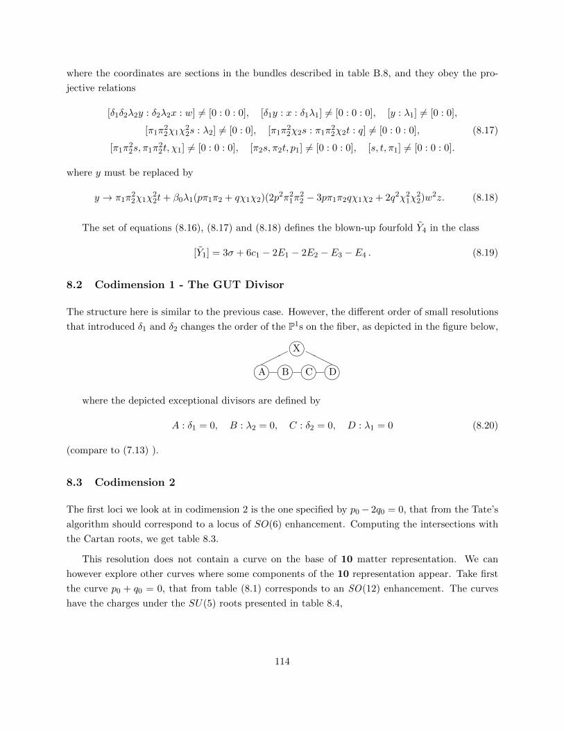
where the coordinates are sections in the bundles described in table B.8, and they obey the pro-
jective relations
[δ1δ2λ2y : δ2λ2x : w] 6= [0 : 0 : 0], [δ1y : x : δ1λ1] 6= [0 : 0 : 0], [y : λ1] 6= [0 : 0],
[π1π22χ1χ
22s : λ2] 6= [0 : 0], [π1π
22χ2s : π1π
22χ2t : q] 6= [0 : 0 : 0], (8.17)
[π1π22s, π1π
22t, χ1] 6= [0 : 0 : 0], [π2s, π2t, p1] 6= [0 : 0 : 0], [s, t, π1] 6= [0 : 0 : 0].
where y must be replaced by
y → π1π22χ1χ
22t+ β0λ1(pπ1π2 + qχ1χ2)(2p2π2
1π22 − 3pπ1π2qχ1χ2 + 2q2χ2
1χ22)w2z. (8.18)
The set of equations (8.16), (8.17) and (8.18) defines the blown-up fourfold Y4 in the class
[Y1] = 3σ + 6c1 − 2E1 − 2E2 − E3 − E4 . (8.19)
8.2 Codimension 1 - The GUT Divisor
The structure here is similar to the previous case. However, the different order of small resolutions
that introduced δ1 and δ2 changes the order of the P1s on the fiber, as depicted in the figure below,
HHH
A B C D
X
where the depicted exceptional divisors are defined by
A : δ1 = 0, B : λ2 = 0, C : δ2 = 0, D : λ1 = 0 (8.20)
(compare to (7.13) ).
8.3 Codimension 2
The first loci we look at in codimension 2 is the one specified by p0− 2q0 = 0, that from the Tate’s
algorithm should correspond to a locus of SO(6) enhancement. Computing the intersections with
the Cartan roots, we get table 8.3.
This resolution does not contain a curve on the base of 10 matter representation. We can
however explore other curves where some components of the 10 representation appear. Take first
the curve p0 + q0 = 0, that from table (8.1) corresponds to an SO(12) enhancement. The curves
have the charges under the SU(5) roots presented in table 8.4,
114

Curve Charges Weights
Ap−2q (-2,1,0,0,1) −α1
Bp−2q (1,-2,1,0,0) −α2
C1 p−2q (0,1,-1,0,0) −µ5 + α1 + α2
C2 p−2q (0,0,-1,1,0) µ5 − α1 + α2 − α3
Dp−2q (0,0,1, -2, 1) −α4
Xp−2q (1,0,0,1,-2) −α5
Table 8.3: Curves and their respective weights at the pπ1π2 − 2qχ1χ2 = 0 locus. The definingequations are presented in table B.10.
Curve Charges Weights
A1 p−q (-2,1,0,0,1) −α1
A2 p−q (0,1,0,-2,1) −α1 + 2(µ10 − α2 − α3 − α4)
A3 p−q (-1,0,0,1,0) −µ10 + α2 + α3 + α4
Bp−q (1,-2,1,0,0) −α2
C1 p−q (0,-2,1,1,0) −α3 + 3(µ5 − α1 − α2)
C2 p−q (0,1,-1,0,0) −µ5 + α1 + α2
C3 p−q (0,1,-1,0,0) −µ5 + α1 + α2
Dp−q (0,0,1, -2, 1) −α4
Xp−q (1,0,0,1,-2) −α0
Table 8.4: Charges and weights of curves at the p0 − q0 = 0
Similarly as we had in the first resolution 7, the curves at the p0 − q0 = 0 locus of the base
reproduce the 5 + 10 representation. The charges are not being conserved, as one can check that
A → A1 p−q +A2 p−q +A3 p−q , (8.21)
C → C1 p−q + C2 p−q + C3 p−q , (8.22)
while the multiplicities fail to reproduce these splitting.
Another interesting locus is the “E6” enhancement curve, given by p0 = 0 (or q0 = 0). The
charges of the fiber curves appearing there are given by table 8.5.
If we look also at the curves of zero charge, at this locus some solutions are not simple P1s
inside the resolved elliptic curve, as before. Take as an example the curve B before restricting to
the p0 locus. Along the p0 = π1π2q = 0 locus, β4 and β5 vanish, so the defining equation of the
curve simplifies to
δ2 = π1π22χ1χ
22s(π1π
22χ1χ
22t+ λ1β3w
2) + λ1λ2(−δ21λ
21w
5 + δ1λ1β2w2x) = δ1t = 0. (8.23)
However the restriction to the E6 curve can be taken to be p = 0, π1 = 0 or π2 = 0. When
π1 = 0 the curve B reduces to
(π1 = 0) δ2 = δ1λ21λ2(−δ1λ1w
5 + β2w2x) = δ1t = 0. (8.24)
115
That has as one possible solution
E∗ : δ2 = π1 = δ1 = 0. (8.25)
The rescaling conditions that have to be obeyed for E∗ are
[0 : 0 : w], [0 : x : 0], [λ1qχ1χ2wz : λ1], [0 : λ2], [0 : 0 : q], [0 : 0 : χ1], [π2s : π2t : p], , [s : t : 0].
Using the fact that χ1χ2q 6= 0 and the rescaling conditions above, we can fix χ1 = q = λ2 = x =
w = λ1 = 1, and we are still left with the unfixed coordinates π2, s, t and q, together with the
conditions
[π2s : π2t : p], [s : t]. (8.26)
So, the solution E∗ is actually a P2 specified by the coordinates and rescaling [s′ : t′ : p] blown up
at the point s′ = t′ = 0 by a P1.
There are however minimal solutions that correspond to a P1 hypersurface inside this P2. As
one concrete example, take the intersection of B with p = 0,
(p =)δ2 = π1π22χ1χ
22s(π1π
22χ1χ
22t+ λ1(qχ1χ2)3w2) + δ1λ
21λ2w
2(−δ1λ1w3 + 3(qχ1χ2)2x) = δ1t = 0,
(8.27)
that has as one possible solution
E∗p : (p =)δ2 = δ1 = π1 = 0. (8.28)
We can see from the defining equations of E∗ (8.25) and (8.26) that E∗p is a P1 hypersurface inside
E∗.
In the M-theory perspective, the four-cycle P2 can be wrapped by M5-branes that correspond
to a string in the remaining dimensions with tension given by the volume of the four-cycle [186].
When shrunken back to zero volume, the wrapped M5-branes become tensionless strings. In the
effective theory, this corresponds to a tensor multiplet becoming massless, leading to a breaking of
Curve Charges Weights
A1 p (0,1,0,-2,1) −α4 + (µ5 − α1 − α2)
A2 p (-2,1,0,0,1) −α1
Bp (1,-2,1,0,0) −α2
C1 p (0,1,-1,0,0) µ5 − α1 − α2
C2 p (0,0,-1,1,0) −µ5 + α1 + α2 + α3
C3 p (0,0,-1,1,0) −µ5 + α1 + α2 + α3
Dp (0,0,1, -2, 1) −α4
Xp (1,0,0,1,-2) −α0
Table 8.5: Curves of non-vanishing charges along the p0 = 0 locus.
116

the low-energy effective theory and thus a phase transition. In the Type IIB picture, the blow-up
introduce a one dimensional P1 on the fiber and also a P1 on the base along the matter curve (one
non-trivially fibered over the other). This blown-up P1 can be wrapped by a D3-brane, that again
in the blown-down limit give rise to a massless string. Additionally, we might have to worry about
string worldsheet instantons wrapping the vanishing P1s. The P1 along the curve might also break
the Calabi-Yau condition. A similar blow-up along a curve in Type IIB picture was studied in [13].
A more detailed exploration of the role of tensionless strings on the theory (or the phase transition)
arising in this particular setup would be interesting, however we do not deal with it in this work.
8.4 Codimension 3
We next restrict the elliptic fiber to the Yukawa point, that before the blow ups corresponded to the
locus w0 = p0 = q0 = 0. Similarly, the restriction to the codimension three locus has as solutions
some curves that are not P1s, but again, some of the internal P1 hypersurfaces appear as solutions.
The calculations of the corresponding charges give the table 8.6.
Curve Charges
A1 E8 (-2,1,0,0,1) −α1
A2 E8 (0,1,0,-2,1) −α4 + (−µ5 + α1 + α2)
BE8 (1,-2,1,0,0) −α2
C1 E8 (0,1,-1,0,0) µ5 − α1 − α2
C2 E8 (0,0,-1,1,0) −µ5 + α1 + α2 + α3
C3 E8 (0,-2,1,1,0) −α3 + 3(−µ5 + α1 + α2)
DE8 (0,0,1, -2, 1) −α4
XE8 (1,0,0,1,-2) −α0
Table 8.6: Curves of non-vanishing charges along the p0 = q0 = 0 locus.
8.5 The p↔ q symmetry
The monodromies present among the matter curves can lead to constrains to the couplings. In the
present model we see a clear symmetry under exchange of p ↔ q, that thus corresponds to the
interchange
(t1, t2, t3, t4, t5)→ (t2, t1, t3, t5, t4), (8.29)
with the tis specified in (8.1). This is similar to the Z2 × Z2 symmetry as the ones described
for example in [16, 187]. We can then restrict the number of families by their orbits under the
117
symmetry group,
Orb(5(1)) : p+ q
Orb(5(2)) : p, q
Orb(5(3)) : p+ 2q, q + 2p
Orb(5(4)) : p− 2q, q − 2p (8.30)
Orb(5(5)) : p− q, q − p
Orb(10(1)) : p+ q
Orb(10(2)) : p, q.
The fact that 10(1) and 10(2) lie in the same matter curve as 5(1) and 5(2), respectively, further
restrict the possible superpotential couplings we can construct in this model.
9 Conclusions
We use the Griffiths-Frobenius structure and homological mirror symmetry to construct an integer
monodromy basis on the primitive horizontal subspace of Calabi-Yau fourfolds together with a
pairing η that determines the Kahler potential in the complex moduli space. For all hypersurfaces
and complete intersections this yields a general method to obtain the exact expressions for periods
that converge at large radius limits with a radius of convergence that is limited by the distance
to the generic conifold divisor. We confirmed this method by comparison with the results of
supersymmetric localization on the hemi-sphere with supersymmetric boundary condition by Hori
and Romo [100]. In particular one can specify boundary data that describe a basis of A-model
branes that correspond to twisted line bundles. The formalism of [100] allows to write down a
preferred Mellin-Barnes integral representation for the corresponding basis of B-model periods,
which relate roughly two regions in the moduli space: the large radius and the Landau Ginzburg
region. Homological mirror symmetry and the Hirzebruch Riemann Roch formula yield the pairing
η for these K-theory classes. This basis does not correspond to a minimal integer monodromy basis
as can be seen from the rational entries in m in (3.139-3.142). The relative factor is crucial. e.g.
for the determination of the actual chiralities in F-theory.
In conjunction with the ideal of Picard-Fuchs equations our method of determining the integer
monodromy basis allows to give convergent expression for the periods everywhere in the moduli
space and therefore to obtain exact expressions of the superpotential and the Kahler potential in all
regions of the vev’s of the N = 1 scalar fields. Even more basic, but quite important for F-theory
phenomenology, it determines the correct N = 1 coordinates in which the effective action is locally
parametrized. This is natural for the complex deformations, but mirror symmetry extends the
method to the complexified Kahler parameters. These periods have very interesting arithmetic and
118

modular properties. Because of the occurrence of closed and open moduli in the fourfold periods
they imply interesting analytic relations between open and closed amplitudes.
We show in detail that the complex moduli can be stabilized by the G4-form superpotential at
orbifold points and that different than in the threefold case for suitable fluxes the scalar potential
for the complex fields vanishes. This behaviour occurs generically in F-theory vacua described
by Fermat hypersurfaces. We also analyze the super potential and the Kahler potential close the
most generic singularity of a Calabi-Yau fourfold, where S4 cycles shrink and a Z2 singularity
appears and show that a flux on the vanishing period can drive the theory to the Z2 orbifold point.
For the generic conifold discriminant of the GKKZ system, homological mirror symmetry maps
this vanishing cycle to the structure sheaf of the mirror manifold. This information in conjunction
with Griffiths transversality allows to see that the Γ-classes give the right modification of the Chern
character map to yield an integer monodromy basis and the right central charges for the Bridgeland
stability conditions [131].
Symmetries on the Calabi-Yau manifold Mn give rise to symmetries in the moduli space Mcs.
Based on the latter symmetries and the local behaviour of the periods at the invariant sublocus
S we describe the conditions under which one can find an integral flux that drives the moduli of
the theory to the invariant sublocus S, with and without creating a potential on S. The Hodge
bundle H restricted to S carries a sub-monodromy problem. In particular for Calabi-Yau manifolds
embedded as hypersurfaces into toric ambient spaces given by a pair of reflexive polyhedra (∆,∆∗)
one can characterize certain sub-mondromy problems and the locus S by reflexive pairs (∆,∆∗)
with the embedding condition∆ ⊂ ∆. This yields a restricted ideal of Picard Fuchs operators
defining the sub-mondromy problem on H|S . We argue that one pick always an integer flux that
creates a potential with S as vacuum manifold. The two constructions have an overlap, because in
many cases∆ can be readily defined by the monomials that are invariant under a symmetry in P∆
that acts also on Mn.
Classical mirror symmetry is obviously useful for determining the holomorphic F-theory am-
plitudes. Mirror symmetry in the tt∗ structures could extend the predictions beyond these terms.
Homological mirror symmetry played a small role in our analysis, but there are very interesting
much further reaching observations. For example for the Hitchin systems with gauge groups G
it has been observed that homological mirror symmetry can be identified with Langland’s duality
exchanging G with the Langland’s dual group G, see [188] for a review. These Hitchin system
arise in the limit of F-theory compactifications and for these cases Langland’s duality is implied
by homological mirror symmetry on fourfolds. The ubiquitous occurrence of modular forms in the
amplitudes on fourfolds, when expressed in the right coordinates, resonates well with these obser-
vations. In particular the superpotential and the scalar potential, that we can calculate everywhere
in the moduli space inherit these modular properties and it would be interesting to make a serious
study of axion inflation based on these exact expressions.
119

In Section 4.1 we construct families of toric hypersurfaces to give global Calabi-Yau 4-folds with
elliptic fibrations of type D5, E6, E7 and E8, and the most general complex structure, which can be
specialized by turning on G4 fluxes. In this way singularities in different co-dimensions are obtained
yielding non-abelian gauge symmetry enhancements, matter curves and Yukawa couplings.
Starting in Section 6 we constructed two models that contained a codimension 3 locus with an
E8 singularity. First, we discuss how a codimension 3 E8 singularity can be embedded in some
of the studied global models. We imported results from F-theory/Heterotic duality, specially the
identification via the spectral cover of the coefficients in the elliptic fiber with the vevs for the Higgs
field responsible for breaking the E8 gauge group in SU(5) with the desired higher codimension
enhancements.
To fully resolve the space, we had to perform blow-ups that introduced two(-complex)-dimensional
subspaces along the codimension two enhancement loci. After resolving, we identified the enhance-
ment loci of the two models and calculated the charges under the SU(5) group, identifying the
associated weights of 5 and 10. We argued that some curves in our particular choice of moduli
carry a 5 + 10 representation.
Also, we show that both the models presented do not give an E8 Dynkin diagram after resolving
the E8 point. Similar feature appears with the codimension 2 locus of E6 singularity, but is not
observed when the singularities are of SO(2n) or SU(n) types. It appears to us that the mismatch
between the expected fiber structure of the resolved space and the type of singularity is a feature
of the strong coupling of the exceptional Ek kinds.
Acknowledgments
We would like to thank Victor Batyrev, Marcos Marino, Emanuel Scheidegger and Stefan Theisen
for correspondences and Sergei Galkin, Daniel Huybrecht, Sheldon Katz, Duco van Straten and
Yongbin Ruan for mathematical advises. We benefited from discussion with Pedro Acosta, Babak
Haghighat, Sven Krippendorf, Maximilian Poretschkin, Dustin Ross, and Timo Weigand. Spe-
cial thanks to Kentaro Hori, Hiroshi Irritani, Hans Jockers and Denis Klevers for many useful
conversations and explanations of their work.
A.K. and D.V.L. are supported by the DFG grant KL 2271/1-1, D.V.L. wants to thank the
Haussdorff Institut for hospitality and support. D.V.L. was also supported by the PDJ fellow-
ship of CNPq, grant number 501107/2012-6. N.C.B. wants to thank for support by a PROMEP
postdoctoral grant, the SFB-Tansregio TR33 “The Dark Universe” (DFG), the EU 7th network pro-
gram “Unification in the LHC era” (PITN-GA-2009-237920), CEADEN and “Proyecto de Ciencias
Basicas: Teorıa Cuantica de Campos en Fısica de Partıculas y de la Materia Condensada” ICIMAF,
CITMA.
120

This work was finished while A.K enjoyed the hospitality of MCTP in the Physics Department
and the Mathematics Department of the University of Michigan in Ann Arbor, supported by the
DMS grant DMS1159265.
A Gauge symmetries enhancements for E8, E7 and E6 fiber types.
All the fiber types E6 × U(1)2, E7 × U(1) and E8 can be brought to the Weierstrass form. In
table A.1 we have summarized Kodaira classification of codimension 1 singularities. Using the
given information one can obtain the monodromies using Tate’s algorithm. In the following we will
describe the obtained enhancement for the different cases.
Type ord(f) ord(g) ord(∆) a j(τ) Group Monodromy
I0 ≥ 0 ≥ 0 0 0 R —
(0 1−1 0
)I1 0 0 1 1
12 ∞ U(1)
(1 10 1
)In 0 0 n > 1 n
12 ∞ An−1
(1 n0 1
)II ≥ 1 1 2 1
6 0 —
(1 1−1 0
)III 1 ≥ 2 3 1
4 1 A1
(0 1−1 0
)IV ≥ 2 2 4 1
3 0 A2
(0 1−1 −1
)I∗n
2 ≥ 3n+ 6 1
2 + n12 ∞ Dn+4
(−1 −b0 −1
)≥ 2 3
IV ∗ ≥ 3 4 8 23 0 E6
(−1 −11 0
)III∗ 3 ≥ 5 9 3
4 1 E7
(0 −11 0
)II∗ ≥ 4 5 10 5
6 0 E8
(0 −11 1
)
Table A.1: Kodaira Classification of singular fibers of an K3 elliptic fibration. Table extracted from[14, 35, 157].
A.1 The E8 fibre and Tate’s algorithm
In Table A.2 we have represented the so called non-split cases, which are enhancements that occur
only for a given vanishing order of the coefficients ai and the discriminant ∆, those are the more
generic cases. In addition, when an extra polynomial factorization occurs one obtains the split
enhancements [35]. We have checked which of those cases are realized in the global toric construction
with polytop 1 in figure 1 and no twisting. In this case the vectors ν(i)∗ in (4.6) are given by u1 =
121
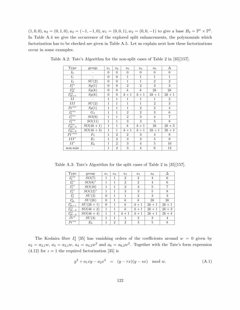
(1, 0, 0), u2 = (0, 1, 0), u3 = (−1,−1, 0), w1 = (0, 0, 1), w2 = (0, 0,−1) to give a base B3 = P1 × P2.
In Table A.4 we give the occurrence of the explored split enhancements, the polynomials which
factorization has to be checked are given in Table A.5. Let us explain next how these factorizations
occur in some examples.
Table A.2: Tate’s Algorithm for the non-split cases of Table 2 in [35][157].
Type group a1 a2 a3 a4 a6 ∆
I0 – 0 0 0 0 0 0
I1 – 0 0 1 1 1 1
I2 SU(2) 0 0 1 1 2 2
Ins3 Sp(1) 0 0 2 2 3 3
Ins2k Sp(k) 0 0 k k 2k 2k
Ins2k+1 Sp(k) 0 0 k + 1 k + 1 2k + 1 2k + 1
II – 1 1 1 1 1 2
III SU(2) 1 1 1 1 2 3
IV ns Sp(1) 1 1 1 2 2 4
I∗ns0 G2 1 1 2 2 3 6
I∗ns1 SO(9) 1 1 2 3 4 7
I∗ns2 SO(11) 1 1 3 3 5 8
I∗ns2k−3 SO(4k + 1) 1 1 k k + 1 2k 2k + 3
I∗ns2k−2 SO(4k + 3) 1 1 k + 1 k + 1 2k + 1 2k + 4
IV ∗ns F4 1 2 2 3 4 8
III∗ E7 1 2 3 3 5 9
II∗ E8 1 2 3 4 5 10
non-min – 1 2 3 4 6 12
Table A.3: Tate’s Algorithm for the split cases of Table 2 in [35][157].
Type group a1 a2 a3 a4 a6 ∆
I∗ss0 SO(7) 1 1 2 2 4 6
I∗s0 SO(8)∗ 1 1 2 2 4 6
I∗s1 SO(10) 1 1 2 3 5 7
I∗s2 SO(12)∗ 1 1 3 3 5 8
Is3 SU(3) 0 1 1 2 3 3
Is2k SU(2k) 0 1 k k 2k 2k
Is2k+1 SU(2k + 1) 0 1 k k + 1 2k + 1 2k + 1
I∗s2k−3 SO(4k + 2) 1 1 k k + 1 2k + 1 2k + 3
I∗s2k−2 SO(4k + 4) 1 1 k + 1 k + 1 2k + 1 2k + 4
IV s SU(3) 1 1 1 2 3 4
IV ∗s E6 1 2 2 3 5 8
The Kodaira fiber Is3 [35] has vanishing orders of the coefficients around w = 0 given by
a2 = a2,1w, a3 = a3,1w, a4 = a4,2w2 and a6 = a6,2w
2. Together with the Tate’s form expression
(4.12) for z = 1 the required factorization [35] is
y2 + a1xy − a2x2 = (y − rx)(y − sx) mod w. (A.1)
122

Table A.4: Toric CY realization with no twisting ni = 0 in (4.6), of split cases from Table 2 in [35].(X) means that the model is realized with the splitting, (dns) means that it does not split. (aut)means that there is an additional automorphism, which reduces h11 and (as) means that there areadditional singularities due to the global constraints. The latter lead to extra h11 forms. A13 isthe last case in the Ak series with [ai] = [0, 1, 6, 7,∞] and D13 is the last case in the Dk series with[ai] = [1, 1, 6, 7,∞]. Above this k the polyhedra are not reflexive.
Type group χ h11 h31 h2,1 Com.
Is4 SU(4) 14328 6 3277 0 XIs5 SU(5) 12978 7 2148 0 XIs6 SU(6) 11682 8 1931 0 XIs7 SU(7) 10332 9 1705 0 XIs8 SU(8) 9036 10 1488 0 XIs9 SU(9) 7686 11 1262 0 XIs10 SU(10) 6390 12 1245 0 XIs11 SU(11) 5040 13 819 0 XIs12 SU(12) 3744 14 602 0 XIs13 SU(13) 2232 16 348 0 X as (1)
IV s SU(3) 15624 5 2591 0 XI∗ss0 SO(7) 14328 6 2374 0 dns
I∗s0 SO(8)∗ 14328 6 2374 0 dns aut (-1)
I∗s1 SO(10) 12924 8 2138 0 XI∗s2 SO(12)∗ 12924 8 2138(55) 0 dns aut (-1)
I∗s3 SO(14) 10224 11 1695 10 XI∗s4 SO(16) 10224 11 1695(55) 10 dns
I∗s5 SO(18)∗ 7524 14 1252 20 X (+2)
I∗s6 SO(20) 7524 14 1252(55) 20 dns (+1)
I∗s7 SO(22) 10224 17 809 30 X (+3)
I∗s8 SO(24) 10224 17 809(55) 30 dns (+2)
I∗s9 SO(26) 1962 21 338 40 X (+5)
IV ∗s E6 12762 9 2110 0 X
We find that (4.12) at z = 1 can be written as (A.1) with r and s given by
2r = −a1 ∓√a2
1 + 4a2 = −a1 ∓√χ2 +O(w) = −a1 ∓ χ+
1
2O(w),
2s = −a1 ±√a2
1 + 4a2 = −a1 ±√χ2 +O(w) = −a1 ± χ+
1
2O(w).
Therefore in a vicinity of w = 0 a factorization of (A.1) involving analytic functions r and s occurs
mod w :
y2 + a1xy − a2x2 =
(y − 1
2(−a1 ∓ χ)x
)(y − 1
2(−a1 ± χ)x
)mod w, (A.2)
with
χ = w2(u31 + u2
1u2 + u1u22 + u3
2 + u21u3 + u1u2u3 + u2
2u3 + u1u23 + u2u
23 + u3
3). (A.3)
In the sum from (A.3) we have omitted the moduli coefficients, so let us make clear that this
factorization occurs without fixing the moduli. This situation is also found for the fibers Is4 , Is5 , Is6
123

and Is7 represented in Table A.4, and the factorization occurs exactly in the same way. The table
A.5 gives the list of polynomials on which the non-split, split and semi-split cases occur.
Table A.5: In the first column the Kodaira fiber type is given, the second column represents thegauge symmetry and in the last column the polynomials that need to factorize to have the splitgauge enhancements are given[35].
Kodaira fiber Group Equation
Ins2k , Is2k Sp(k), SU(2k) Y 2 + a1XY − a2X
2
Ins2k+1, Is2k+1 unconven., SU(2k + 1) Y 2 + a1XY − a2X
2
I∗ns0 , I∗s0 , I∗ss0 G2, SO(8)∗, SO(7) X3 + a2,1X2 + a4,2X + a6,3
I∗s0 SO(8)∗ X2 + a2,1X + a4,2
I∗ns2k−2, I∗s2k−2 SO(4k + 3), SO(4k + 4)∗, k ≥ 2 a2,1X
2 + a4,k+1X + a6,2k+1
I∗ns2k−3, I∗s2k−3 SO(4k + 1), SO(4k + 2) Y 2 + a3,kY − a6,2k
IV ∗ns, IV ∗s F4, E6 Y 2 + a3,2Y − a6,4
IV ns, IV s unconven., SU(3) Y 2 + a3,1Y − a6,2
Let us see the remaining cases. For I∗s1 the factorization that has to occur is the one of the
polynomial Y 2 + a3,2Y − a6,4. Around v = 0, this can be seen from the roots, that appear when
a23,2 + 4a6,4 is a square. Here we obtain
a23,2 + 4a6,4 = w8(u9
1 + u81u2 + u7
1u22 + u6
1u32 + u5
1u42 + u4
1u52 + u3
1u62 + u2
1u72 + u1u
82 (A.4)
+u92 + u8
1u3 + u71u2u3 + u6
1u22u3 + u5
1u32u3 + u4
1u42u3 + u3
1u52u3 + u2
1u62u3
+u1u72u3 + u8
2u3 + u71u
23 + u6
1u2u23 + u5
1u22u
23 + u4
1u32u
23 + u3
1u42u
23 + u2
1u52u
23
+u1u62u
23 + u7
2u23 + u6
1u33 + u5
1u2u33 + u4
1u22u
33 + u3
1u32u
33 + u2
1u42u
33 + u1u
52u
33
+u62u
33 + u5
1u43 + u4
1u2u43 + u3
1u22u
43 + u2
1u32u
43 + u1u
42u
43 + u5
2u43 + u4
1u53
+u31u2u
53 + u2
1u22u
53 + u1u
32u
53 + u4
2u53 + u3
1u63 + u2
1u2u63 + u1u
22u
63
+u32u
63 + u2
1u73 + u1u2u
73 + u2
2u73 + u1u
83 + u2u
83 + u9
3)2 ,
omitting the moduli coefficients. And the split singularity occurs in our construction. The same
occurs for I∗s3 , where Y 2 + a3,3Y − a6,6 factorizes because a23,3 + 4a6,6 is a square proportional to
(A.4). The same occurs for the case I∗s5 where a23,4 + 4a6,8 is a square proportional to (A.4) giving
a factorization of Y 2 + a3,4Y − a6,8.
The other realized split case is the singularity IV ∗, which appears when (Y 2 + a3,2Y − a6,4)
factorizes. This happens when a23,2 + 4a6,4 is a square in the vicinity of v = 0, and this is the case
because is identical to (A.4).
For I∗0 the polynomial which needs to be analyzed is
X3 + a2,1X2 + a4,2X + a6,3. (A.5)
There are the cases non-split, semi-split or split, depending on wether (A.5) is non-factorizable,
factorizable in terms of linear and quadratic terms or factorizable in three linear terms. The model
124

in this appendix only accommodates the non-split case generically. Also for the case I∗s0 with group
SO(8), the moduli need specification to obtain the factorization of (X2 +a2,1X+a4,2), which occurs
when a22,1 − 4a4,2 is a square. The same happens for the singularity I∗s2 which can also not been
obtained generically. The study presented is partial, but with our construction we have the tools
to explore systematically by varying the data of the Calabi-Yau, whether the split enhancements
not realized here appear generically in other models.
A.2 Codimension 1 singularities for E7 × U(1) and the E6 × U(1)2 fibre .
In this section we give the list of codimension 1 enhancements for the E7×U(1) fiber as well as the
E6×U(1)2. In the tables A.6 and A.6 every column gives the vanishing order of the coefficients of
the elliptic fibration equation in terms of a coordinate u1, such that at u1 = 0 the given singularity
appears. Furthermore for the toric CY construction embedding the singularities, we consider the
basis B2 = P1 and B3 = P3, following the vanishing orders of the coefficients the properties of the
3-fold and 4-fold are given.
125

Table A.6: A list of vanishing order of the coefficients in (5.23) and the corresponding singularityfor the E7 × U(1) fiber.
Singularity a3 a2 b2 a1 a0 χ3 h311 h3
21 χ4 h411 h4
31 h421
D0 ≥ 1 ≥ 1 ≥ 1 ≥ 2 2 -228 6(0) 120(4) 6612 6(0) 1088(15) 0D0 ≥ 1 1 1 ≥ 2 3 -208 7(0) 111(0) 6024 7(0) 989(0) 0D1 ≥ 1 1 ≥ 2 ≥ 2 3 -208 7(0) 111(6) 6024 7(0) 989(36) 0D1 ≥ 1 ≥ 2 1 2 3 -194 8(0) 105(0) 5814 8(0) 953(0) 0D1 ≥ 1 1 ≥ 2 2 4 -180 8(0) 98(0) 5244 8(0) 858(0) 0D2 ≥ 1 ≥ 2 1 ≥ 3 3 -176 9(0) 97(0) 5424 9(0) 887(0) 0D2 ≥ 1 1 ≥ 2 ≥ 3 4 -160 13(4) 93(3) 4824 9(0) 802(10) 15D2 ≥ 1 2 1 ≥ 3 4 -156 14(4) 92(0) 4878 10(0) 810(0) 15D2 ≥ 1 1 2 ≥ 3 5 -144 14(4) 86(0) 4392 10(0) 729(0) 15A1 ≥ 0 1 0 ≥ 1 1 -280 4(0) 144(0) 8064 4(0) 1332(0) 0A1 ≥ 0 0 ≥ 1 ≥ 1 2 -264 4(0) 136(0) 7338 4(0) 1211(0) 0A2 0 ≥ 1 ≥ 1 1 2 -248 5(0) 129(0) 7074 5(0) 1166(0) 0A3 ≥ 0 ≥ 2 0 ≥ 2 2 -240 5(0) 125(2) 6804 5(0) 1121(3) 0A3 0 ≥ 2 ≥ 1 ≥ 2 2 -228 6(0) 120(0) 6612 6(0) 1088(0) 0A3 0 1 1 ≥ 2 3 -218 6(0) 115(0) 6108 6(0) 1004(0) 0A3 ≥ 0 0 ≥ 2 ≥ 2 4 -212 5(0) 111(2) 5604 5(0) 921(3) 0A4 0 ≥ 2 1 2 3 -204 7(0) 109(0) 5898 7(0) 968(0) 0A4 0 1 ≥ 2 2 4 -190 7(0) 102(0) 5328 7(0) 873(0) 0A5 ≥ 0 ≥ 3 0 ≥ 3 3 -204 6(0) 108(4) 5712 6(0) 938(6) 0A5 0 ≥ 3 1 ≥ 3 3 -186 8(0) 101(0) 5508 8(0) 902(0) 0A5 0 2 1 ≥ 3 4 -176 8(0) 96(0) 5046 8(0) 825(0) 0A5 0 ≥ 2 ≥ 2 2 4 -176 8(0) 96(0) 5118 8(0) 837(0) 0A5 ≥ 0 0 ≥ 3 ≥ 3 6 -168 6(0) 90(4) 4254 6(0) 695(6) 0A5 0 2 ≥ 2 ≥ 3 4 -164 11(2) 93(0) 4878 9(0) 799(0) 3A5 0 1 2 ≥ 3 5 -164 8(0) 90(0) 4560 8(0) 744(0) 0A6 0 ≥ 3 1 3 4 -164 9(0) 91(0) 4884 9(0) 797(0) 0A6 0 3 ≥ 2 3 4 -152 12(2) 88(0) 4716 10(0) 771(0) 3A6 0 2 2 3 5 -144 12(2) 84(0) 4338 10(0) 708(0) 3A6 0 1 ≥ 3 3 6 -140 9(0) 79(0) 3966 9(0) 644(0) 0A7 ≥ 0 ≥ 4 0 ≥ 4 4 -172 7(0) 93(6) 4776 7(0) 781(9) 0A7 0 ≥ 4 1 ≥ 4 4 -148 10(0) 84(0) 4560 10(0) 742(0) 0A7 0 3 1 ≥ 4 5 -138 10(0) 79(0) 4140 10(0) 672(0) 0A7 0 4 ≥ 2 ≥ 4 4 -136 13(2) 81(0) 4392 11(0) 716(0) 3A7 0 3 2 3 5 -132 13(2) 79(0) 4176 11(0) 680(0) 3A7 0 0 4 4 8 -132 7(0) 73(6) 3240 7(0) 525(9) 0A7 0 3 2 ≥ 4 5 -120 16(4) 76(0) 3960 12(0) 646(0) 6A7 0 2 ≥ 3 3 6 -120 13(2) 73(0) 3744 11(0) 608(0) 3A7 0 2 2 ≥ 4 6 -120 13(2) 73(0) 3672 11(0) 596(0) 3A7 0 1 3 ≥ 4 7 -118 10(0) 69(0) 3372 10(0) 544(0) 0A7 0 2 ≥ 3 ≥ 4 6 -108 16(4) 70(0) 3528 12(0) 574(0) 6E6 ≥ 1 ≥ 2 ≥ 2 2 3 -180 9(0) 99(0) 5604 9(0) 917(0) 0E6 ≥ 1 ≥ 2 ≥ 2 2 4 -152 16(6) 92(0) 4824 10(0) 822(0) 36E7 ≥ 1 ≥ 2 ≥ 2 ≥ 3 3 -144 19(8) 91(0) 4824 11(0) 851(0) 66
126
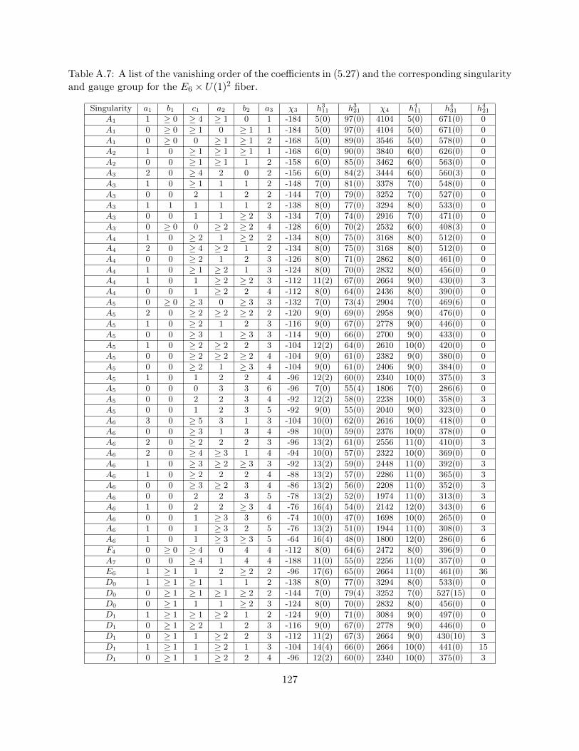
Table A.7: A list of the vanishing order of the coefficients in (5.27) and the corresponding singularityand gauge group for the E6 × U(1)2 fiber.
Singularity a1 b1 c1 a2 b2 a3 χ3 h311 h3
21 χ4 h411 h4
31 h421
A1 1 ≥ 0 ≥ 4 ≥ 1 0 1 -184 5(0) 97(0) 4104 5(0) 671(0) 0
A1 0 ≥ 0 ≥ 1 0 ≥ 1 1 -184 5(0) 97(0) 4104 5(0) 671(0) 0
A1 0 ≥ 0 0 ≥ 1 ≥ 1 2 -168 5(0) 89(0) 3546 5(0) 578(0) 0
A2 1 0 ≥ 1 ≥ 1 ≥ 1 1 -168 6(0) 90(0) 3840 6(0) 626(0) 0
A2 0 0 ≥ 1 ≥ 1 1 2 -158 6(0) 85(0) 3462 6(0) 563(0) 0
A3 2 0 ≥ 4 2 0 2 -156 6(0) 84(2) 3444 6(0) 560(3) 0
A3 1 0 ≥ 1 1 1 2 -148 7(0) 81(0) 3378 7(0) 548(0) 0
A3 0 0 2 1 2 2 -144 7(0) 79(0) 3252 7(0) 527(0) 0
A3 1 1 1 1 1 2 -138 8(0) 77(0) 3294 8(0) 533(0) 0
A3 0 0 1 1 ≥ 2 3 -134 7(0) 74(0) 2916 7(0) 471(0) 0
A3 0 ≥ 0 0 ≥ 2 ≥ 2 4 -128 6(0) 70(2) 2532 6(0) 408(3) 0
A4 1 0 ≥ 2 1 ≥ 2 2 -134 8(0) 75(0) 3168 8(0) 512(0) 0
A4 2 0 ≥ 4 ≥ 2 1 2 -134 8(0) 75(0) 3168 8(0) 512(0) 0
A4 0 0 ≥ 2 1 2 3 -126 8(0) 71(0) 2862 8(0) 461(0) 0
A4 1 0 ≥ 1 ≥ 2 1 3 -124 8(0) 70(0) 2832 8(0) 456(0) 0
A4 1 0 1 ≥ 2 ≥ 2 3 -112 11(2) 67(0) 2664 9(0) 430(0) 3
A4 0 0 1 ≥ 2 2 4 -112 8(0) 64(0) 2436 8(0) 390(0) 0
A5 0 ≥ 0 ≥ 3 0 ≥ 3 3 -132 7(0) 73(4) 2904 7(0) 469(6) 0
A5 2 0 ≥ 2 ≥ 2 ≥ 2 2 -120 9(0) 69(0) 2958 9(0) 476(0) 0
A5 1 0 ≥ 2 1 2 3 -116 9(0) 67(0) 2778 9(0) 446(0) 0
A5 0 0 ≥ 3 1 ≥ 3 3 -114 9(0) 66(0) 2700 9(0) 433(0) 0
A5 1 0 ≥ 2 ≥ 2 2 3 -104 12(2) 64(0) 2610 10(0) 420(0) 0
A5 0 0 ≥ 2 ≥ 2 ≥ 2 4 -104 9(0) 61(0) 2382 9(0) 380(0) 0
A5 0 0 ≥ 2 1 ≥ 3 4 -104 9(0) 61(0) 2406 9(0) 384(0) 0
A5 1 0 1 2 2 4 -96 12(2) 60(0) 2340 10(0) 375(0) 3
A5 0 0 0 3 3 6 -96 7(0) 55(4) 1806 7(0) 286(6) 0
A5 0 0 2 2 3 4 -92 12(2) 58(0) 2238 10(0) 358(0) 3
A5 0 0 1 2 3 5 -92 9(0) 55(0) 2040 9(0) 323(0) 0
A6 3 0 ≥ 5 3 1 3 -104 10(0) 62(0) 2616 10(0) 418(0) 0
A6 0 0 ≥ 3 1 3 4 -98 10(0) 59(0) 2376 10(0) 378(0) 0
A6 2 0 ≥ 2 2 2 3 -96 13(2) 61(0) 2556 11(0) 410(0) 3
A6 2 0 ≥ 4 ≥ 3 1 4 -94 10(0) 57(0) 2322 10(0) 369(0) 0
A6 1 0 ≥ 3 ≥ 2 ≥ 3 3 -92 13(2) 59(0) 2448 11(0) 392(0) 3
A6 1 0 ≥ 2 2 2 4 -88 13(2) 57(0) 2286 11(0) 365(0) 3
A6 0 0 ≥ 3 ≥ 2 3 4 -86 13(2) 56(0) 2208 11(0) 352(0) 3
A6 0 0 2 2 3 5 -78 13(2) 52(0) 1974 11(0) 313(0) 3
A6 1 0 2 2 ≥ 3 4 -76 16(4) 54(0) 2142 12(0) 343(0) 6
A6 0 0 1 ≥ 3 3 6 -74 10(0) 47(0) 1698 10(0) 265(0) 0
A6 1 0 1 ≥ 3 2 5 -76 13(2) 51(0) 1944 11(0) 308(0) 3
A6 1 0 1 ≥ 3 ≥ 3 5 -64 16(4) 48(0) 1800 12(0) 286(0) 6
F4 0 ≥ 0 ≥ 4 0 4 4 -112 8(0) 64(6) 2472 8(0) 396(9) 0
A7 0 0 ≥ 4 1 4 4 -188 11(0) 55(0) 2256 11(0) 357(0) 0
E6 1 ≥ 1 1 2 ≥ 2 2 -96 17(6) 65(0) 2664 11(0) 461(0) 36
D0 1 ≥ 1 ≥ 1 1 1 2 -138 8(0) 77(0) 3294 8(0) 533(0) 0
D0 0 ≥ 1 ≥ 1 ≥ 1 ≥ 2 2 -144 7(0) 79(4) 3252 7(0) 527(15) 0
D0 0 ≥ 1 1 1 ≥ 2 3 -124 8(0) 70(0) 2832 8(0) 456(0) 0
D1 1 ≥ 1 ≥ 1 ≥ 2 1 2 -124 9(0) 71(0) 3084 9(0) 497(0) 0
D1 0 ≥ 1 ≥ 2 1 2 3 -116 9(0) 67(0) 2778 9(0) 446(0) 0
D1 0 ≥ 1 1 ≥ 2 2 3 -112 11(2) 67(3) 2664 9(0) 430(10) 3
D1 1 ≥ 1 1 ≥ 2 1 3 -104 14(4) 66(0) 2664 10(0) 441(0) 15
D1 0 ≥ 1 1 ≥ 2 2 4 -96 12(2) 60(0) 2340 10(0) 375(0) 3
127

B Defining Equations for the Resolved Fourfolds
In this Appendix we write for reference the defining equations for the resolved fourfolds.
B.1 Case 1
The first case considered 7,
t1 = p, t2 = q, t3 = p+ 2q, t4 = −2p− q, t5 = −2q.
B.1.1 The resolved elliptic fibration
(−δ2λ2χ1x
3 + β0qχ1χ23χ4(−2p3 − 11p2qχ1χ2 − 10pq2χ2
1χ22 − 4q3χ3
1χ32)wx2z
+β0χ1χ2χ23χ4(−3p2 − 4pqχ1χ2 − 5q2χ2
1χ22)δ1λ1w
3xz2 − b0δ21λ
21χ
21χ
32χ
23χ4w
5z3)λ1λ2(
β0pq2χ1χ
23(4p2 + 10pqχ1χ2 + 4q2χ2
1χ22)χ4x (B.1)
+2β0pχ23χ4(−p2 − pqχ1χ2 + q2χ2
1χ22)δ1λ1w
2z + δ1δ2y)yz = 0
with the projective relations
δ1δ22λ1λ2χ
21χ
32χ
53χ
74χ
95y : δ2λ1λ2χ1χ2χ
23χ
34χ
45x : z 6= 0 : 0 : 0
δ1δ22λ2χ
21χ
32χ
53χ
74χ
95y : δ2λ2χ1χ2χ
23χ
34χ
45x : w 6= 0 : 0 : 0,
δ1δ2χ1χ22χ
33χ
44χ
55y : x : δ1λ1χ1χ
22χ
23χ
24χ
25 6= 0 : 0 : 0, (B.2)
δ2χ3χ24χ
35y : λ1 6= 0 : 0, y : λ2χ1χ2χ3χ4χ5 6= 0 : 0, q : λ2 : δ1χ2χ3χ4χ5 6= 0 : 0 : 0,
χ1 : δ1 6= 0 : 0, χ2 : p : δ2χ4χ25 6= 0 : 0 : 0, χ3 : δ2χ5 6= 0 : 0 : χ4 : δ2 6= 0 : 0.
128

B.1.2 Sections
x O(σ + 2c1 − E1 − E2)y O(σ + 3c1 − E1 − E2 − E3 − E4)w O(S2 − E1)z O(σ)λ1 O(E1 − E2 − E3)λ2 O(E2 − E4 − E5)δ1 O(E3 − E5 − E6)δ2 O(E4 − E7 − E8 − E9)q O(Q− E5)χ1 O(E5 − E6)p O(P − E7)χ2 O(E6 − E7)χ3 O(E7 − E8)χ4 O(E8 − E9)χ5 O(E9)β0 O(6c1 − 5S2)
Table B.1: The coordinates and their corresponding bundles for case 1.
B.1.3 Curves in codimension 1
A : δ1 = −χ1δ2λ1λ22x
3 + β0χ1χ23χ4qxz(2pq(2p+ χ1χ2q)(p+ 2χ1χ2q)y−
−λ1λ2(2p3 + 11χ1χ2p2q + 10χ2
1χ22pq
2 + 4χ31χ
32q
3)wx) = 0
B : δ2 = −β0χ23χ4z(χ1qx(λ1λ2(2p3 + 11χ1χ2p
2q + 10χ21χ
22pq
2 + 4χ31χ
32q
3)wx−2pq(2p+ χ1χ2q)(p+ 2χ1χ2q)y) + δ1λ1w
2(χ1χ2λ1λ2(3p2 + 4χ1χ2pq + 5χ21χ
22q
2)wx+2p(p2 + χ1χ2pq − χ2
1χ22q
2)y)z + χ21χ
32δ
21λ
31λ2w
5z2) = 0
C : λ2 = yz(δ1δ2y + 2β0χ23χ4p(χ1q
2(2p+ χ1χ2q)(p+ 2χ1χ2q)x−δ1λ1(p2 + χ1χ2pq − χ2
1χ22q
2)w2z)) = 0
D : λ1 = yz(2β0χ1χ23χ4pq
2(2p+ χ1χ2q)(p+ 2χ1χ2q)x+ δ1δ2y) = 0
X : w = −χ1δ2λ1λ22x
3 + yz(δ1δ2y + 2β0χ1χ23χ4pq
2(2p+ χ1χ2q)(p+ 2χ1χ2q)x) = 0
Table B.2: Divisors in the codimension 1 locus w = 0 after the complete blow up. Every curve has multiplicity 1.
129

B.1.4 Curves in codimension 2
Curve Defining equations
Ap−q : δ1 = δ2λ1λ22χ1x
2 + 9β0q4χ4
1χ32χ
23χ4(3λ1λ2wx+ 2qy)z = 0
B1p−q : δ2 = −9q2χ1x+ δ1λ1w2z = 0
B2p−q : δ2 = −q2χ1(3λ1λ2q2wx+ 2qy) + δ1λ
21λ2w
3z = 0
Cp−q : λ2 = 18β0q5χ4
1χ32χ
23χ4x+ δ1δ2y = 0
Dp−q : λ1 = δ1δ2y + 2β0q3χ3
1χ32χ
23χ4(−9q2χ1x+ δ1λ1w
2z) = 0
Xp−q : w = −δ2λ1λ22x
3 − 18β0q5xyz + δ1δ2y
2z = 0
Table B.3: Codimension 2 locus p0 − q0 = 0. Exceptional divisors split as we approach p0 → q0. Each curve hasmultiplicity 1.
Curve Defining equations Multipl.
A1p+2q : δ1 = λ2 = 0 2
A2p+2q : δ1 = δ2λ2x+ 12β0q4χ3
1χ32χ
23χ4wz = 0 1
Bp+2q : δ2 = 12λ2q4χ2
1x2 + δ1q
2χ1w(9λ1λ2wx− 4qy)z + δ21λ
21λ2w
4z2 = 0 1
Cp+2q : λ2 = δ2y + 4β0λ1q3χ3
1χ32χ
23χ4w
2z = 0 1
Dp+2q : λ1 = δ1 = 0 2
Xp+2q : w = (−λ1λ22χ1x
3 + δ1y2z) = 0 1
Table B.4: Codimension 2 locus p0 + 2q0 = 0.
Curve Defining equations Multipl.
A1p : δ1 = λ2 = 0 2
A2p : δ1 = δ2λ2x+ 12β0q4χ3
1χ32χ
23χ4wz = 0 1
B1p : δ2 = λ2 = 0 2
B2Ap : δ2 = q2χ1x+ δ1λ1w2z = 0 1
B2Bp : δ2 = 4q2χ1x+ δ1λ1w2z = 0 1
Dp : λ1 = δ1 = 0 2
Xp : w = (−λ1λ22χ1x
3 + δ1y2z) = 0 1
Table B.5: Codimension 2 locus p0 = 0.
130

Curve Defining equations Multipl.
Aq : δ1 = δ2 = 0 2
Bq : δ2 = 3λ1λ2p2χ1χ2wx+ 2p3y + δ1λ
21λ2χ
21χ
32w
3z = 0 1
Cq : λ2 = d2y − 2β0λ1p3χ2
3χ4w2z = 0 2
Dq : λ1 = −λ1λ22χ1x
3 + δ1y2z = 0 2
Xp : w = (−λ1λ22χ1x
3 + δ1y2z) = 0 1
Cχ1 : λ2 = δ2y − 2β0λ1p3χ2
3χ4w2z = 0 1
Aχ2 : δ1 = δ2λ1λ22x
2 + 2β0p3q(λ1λ2wx− 2qy)z = 0 = 0 1
Bχ2 : δ2 = qχ1x(λ1λ2wx− 2qy) + δ1λ1w2yz = 0 1
Cχ2 : λ2 = δ1δ2y + 2β0p3(2q2χ1x− δ1λ1w
2z) = 0 1
Dχ2 : λ1 = 4β0p3q2χ1x+ δ1δ2y = 0 1
Table B.6: Codimension 2 locus q0 = 0. We also included for reference the curves that fail to intersect the Cartandivisors.
B.1.5 “Curves” in codimension 3
Curve Defining equations
A“E8” : p = q = 0 δ1 = δ2 = 0
C“E8” : p = q = 0 δ2 = λ2 = 0
D“E8” : p = q = 0 δ1 = λ1 = 0
X“E8” : p = q = 0 w = −λ1λ22χ1x
3 + δ1y2z = 0
A1“E8” : p = q = 0 δ2 = χ1 = 0
A2“E8” : p = χ1 = 0 δ2 = =0
A3“E8” : p = χ1 = 0 λ2 = δ2 = 0
A4“E8” : p = χ2 = 0 δ1 = λ1 = 0
A5“E8” : p = χ2 = 0 δ1 = λ2 = 0
A6“E8” : p = χ2 = 0 δ1 = λ1 = 0
A7“E8” : χ3 = 0 δ1 = λ2 = 0
A8“E8” : χ4 = 0 δ1 = λ2 = 0
A9“E8” : χ5 = 0 δ1 = λ2 = 0
Table B.7: Codimension 3 locus q0 = p0 = 0. note that even though we call the restrictions of the exceptionaldivisors to the fourfold “curves”, note that some of the restrictions have higher dimensionality, as equation (8.25)
.
131

B.2 Case 2
B.2.1 The resolved elliptic fibration
0 = π1π
22χ1χ
22s[π1π
22χ1χ
22t+ λ1(pπ1π2 + qχ1χ2)(2p2π2
1π22 − 3pπ1π2qχ1χ2 + 2q2χ2
1χ22)w2
]+
λ1λ2
[−2pπ1π2qχ1χ2(p2π2
1π22 + 4pπ1π2qχ1χ2 + q2χ2
1χ22)− δ2
1λ21w
5+
δ1λ1(3p2π21π
22 + pπ1π2qχ1χ2 + 3q2χ2
1χ22)w2x− δ2λ2x
3]
0 = 4p2π1q2χ1(pπ1π2 + qχ1χ2) + δ2s− δ1t,
(B.3)
where the coordinates are sections in the bundles given in table B.8, together with the list of
projective relations
[δ1δ2λ2y : δ2λ2x : w] 6= [0 : 0 : 0], [δ1y : x : δ1λ1] 6= [0 : 0 : 0], [y : λ1] 6= [0 : 0],
[π1π22χ1χ
22s : λ2] 6= [0 : 0], [π1π
22χ2s : π1π
22χ2t : q] 6= [0 : 0 : 0], (B.4)
[π2π1s : π2π1t : χ1] 6= [0 : 0 : 0], [π2s : π2t : p] 6= [0 : 0 : 0], [s : t : π1] 6= [0 : 0 : 0].
B.2.2 Sections
x O(σ + 2c1 − E1 − E2)y O(σ + 3c1 − E1 − E2 − E3)t O(σ + 3c1 − E1 − E2 − E3 − E5 − E6 − E7 − E8)s O(σ + 3c1 − E1 − E2 − E4 − E5 − E6 − E7 − E8)w O(S2 − E1)z O(σ)λ1 O(E1 − E3)λ2 O(E2 − E4)δ1 O(E3)δ2 O(E4)p O(S2 − c1 − E7 − E8)q O(S2 − c1 − E5 − E6)χ1 O(E5 − E6)χ2 O(E6)π1 O(E7 − E8)π2 O(E8)β0 O(6c1 − 5S2)
Table B.8: Coordinates and their corresponding bundles for case 2.
132
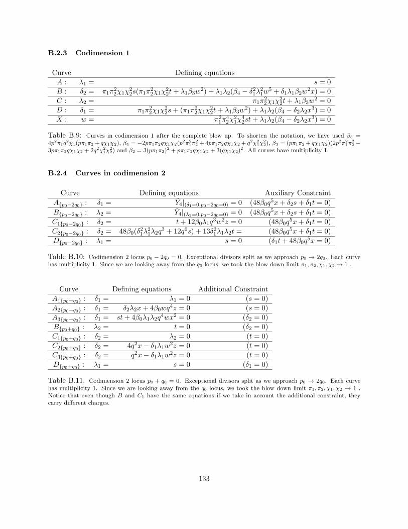
B.2.3 Codimension 1
Curve Defining equations
A : λ1 = s = 0
B : δ2 = π1π22χ1χ
22s(π1π
22χ1χ
22t+ λ1β3w
2) + λ1λ2(β4 − δ21λ
21w
5 + δ1λ1β2w2x) = 0
C : λ2 = π1π22χ1χ
22t+ λ1β3w
2 = 0
D : δ1 = π1π22χ1χ
22s+ (π1π
22χ1χ
22t+ λ1β3w
2) + λ1λ2(β4 − δ2λ2x3) = 0
X : w = π21π
42χ
21χ
42st+ λ1λ2(β4 − δ2λ2x
3) = 0
Table B.9: Curves in codimension 1 after the complete blow up. To shorten the notation, we have used β5 =4p2π1q
2χ1(pπ1π2 + qχ1χ2), β4 = −2pπ1π2qχ1χ2(p2π21π
22 + 4pπ1π2qχ1χ2 + q2χ2
1χ22), β3 = (pπ1π2 + qχ1χ2)(2p2π2
1π22 −
3pπ1π2qχ1χ2 + 2q2χ21χ
22) and β2 = 3(pπ1π2)2 + pπ1π2qχ1χ2 + 3(qχ1χ2)2. All curves have multiplicity 1.
B.2.4 Curves in codimension 2
Curve Defining equations Auxiliary Constraint
Ap0−2q0 : δ1 = Y4|(δ1=0,p0−2q0=0) = 0 (48β0q5x+ δ2s+ δ1t = 0)
Bp0−2q0 : λ2 = Y4|(λ2=0,p0−2q0=0) = 0 (48β0q5x+ δ2s+ δ1t = 0)
C1p0−2q0 : δ2 = t+ 12β0λ1q3w2z = 0 (48β0q
5x+ δ1t = 0)
C2p0−2q0 : δ2 = 48β0(δ21λ
21λ2q
3 + 12q6s) + 13δ21λ1λ2t = (48β0q
5x+ δ1t = 0)
Dp0−2q0 : λ1 = s = 0 (δ1t+ 48β0q5x = 0)
Table B.10: Codimension 2 locus p0 − 2q0 = 0. Exceptional divisors split as we approach p0 → 2q0. Each curvehas multiplicity 1. Since we are looking away from the q0 locus, we took the blow down limit π1, π2, χ1, χ2 → 1 .
Curve Defining equations Additional Constraint
A1p0+q0 : δ1 = λ1 = 0 (s = 0)
A2p0+q0 : δ1 = δ2λ2x+ 4β0wq4z = 0 (s = 0)
A3p0+q0 : δ1 = st+ 4β0λ1λ2q4wx2 = 0 (δ2 = 0)
Bp0+q0 : λ2 = t = 0 (δ2 = 0)
C1p0+q0 : δ2 = λ2 = 0 (t = 0)
C2p0+q0 : δ2 = 4q2x− δ1λ1w2z = 0 (t = 0)
C3p0+q0 : δ2 = q2x− δ1λ1w2z = 0 (t = 0)
Dp0+q0 : λ1 = s = 0 (δ1 = 0)
Table B.11: Codimension 2 locus p0 + q0 = 0. Exceptional divisors split as we approach p0 → 2q0. Each curvehas multiplicity 1. Since we are looking away from the q0 locus, we took the blow down limit π1, π2, χ1, χ2 → 1 .Notice that even though B and C1 have the same equations if we take in account the additional constraint, theycarry different charges.
133

Curve Defining equations Additional Constraint
A1p : δ1 = π1π22t+ 2β0λ1q
3χ21χ2w
2z = 0 (δ2 = 0)
A2p : δ1 = λ1 = 0 (s = 0)
A3p : δ1 = st+ 4β0λ1λ2q4wx2 = 0 (δ2 = 0)
Bp : λ2 = π1π22χ
21χ
42sz(π1π
22t+ 2β0λ1q
3χ21χ2w
2z) = 0 (δ2s− δ1t = 0)
C1p : δ2 = π1π22t+ 2β0λ1q
3χ21χ2w
2z = 0 (δ1 = 0)
C2p : δ2 = s = 0 (δ1 = 0)
C3p : δ2 = 2sπ1π22q
3χ41χ
52 + δ1λ1λ2w(−3q2χ2
1χ22x+ δ1λ1w
2z) = 0 (t = 0)
Dp : λ1 = s = 0 (δ1 = 0)
Table B.12: Codimension 2 locus p0 = 0. Here we have shown only the curves with non-vanishing charges, presentedin table 8.5.
B.2.5 Curves in codimension 3
Curve Defining equations Additional Constraint
A1E8 : δ1 = t = 0 (δ2 = 0)
A2E8 : δ1 = λ1 = 0 (s = 0)
BE8 : λ2 = t = 0 (δ1 = 0)
C1E8 : δ2 = t = 0 (δ1 = 0)
C2E8 : δ2 = s = 0 (δ1 = 0)
DE8 : λ1 = s = 0 (δ1 = 0)
Table B.13: Codimension 3 locus p0 = q0 = 0. Again we present only the curves with non-vanishing charges, fromtable 8.6.
C Calculating the Charges
We calculate the intersections in the same way as in [15, 185]. The coordinates are sections of the
bundles as shown in tables B.1 and B.8, for case 1 and 2, respectively.
In both cases the divisors P and Q are in the same class as S2 − c1.
We then use the projective relations (B.2) and knowing the corresponding bundles of each
section, we can write the vanishing intersections of homology classes. For example, when we
perform the first blow-up
y → λ1y′, x→ λ1x
′, w → λ1w′, (C.1)
We introduced a new divisor E1 defined by λ1 = 0 in the ambient space, and the relation
(σ + 2c1 − E1)(σ + 3c1 − E1)(S2 − E1) = 0. (C.2)
134
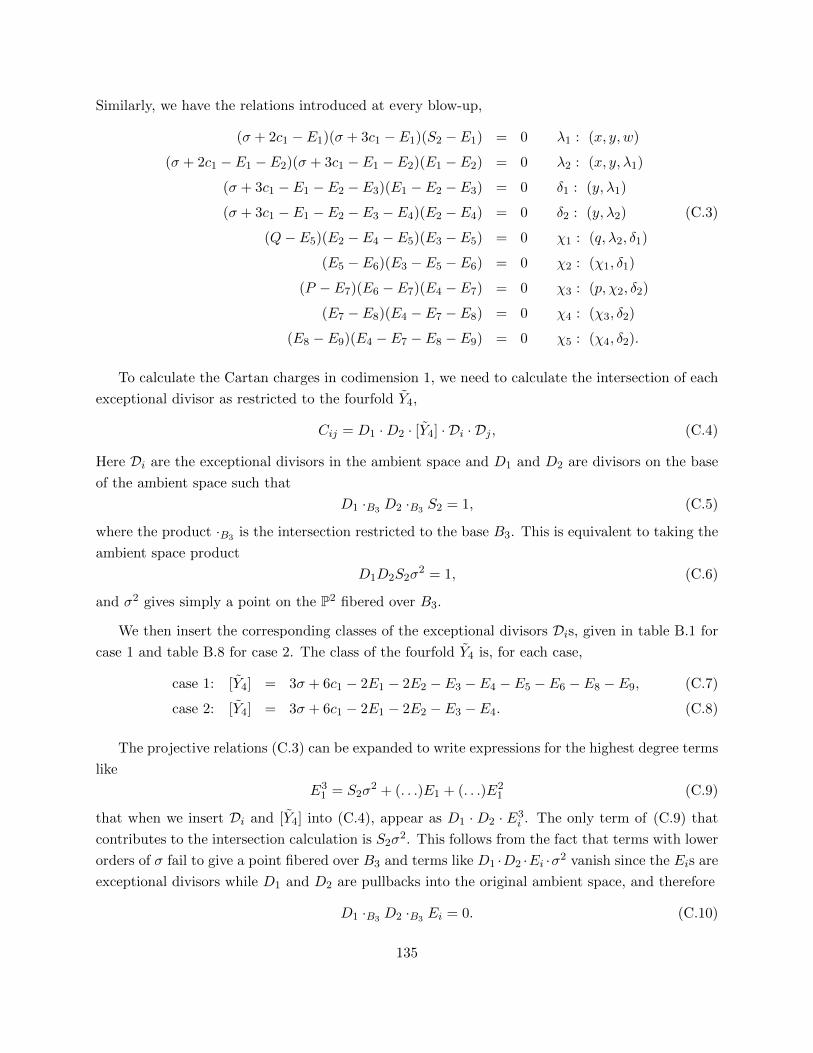
Similarly, we have the relations introduced at every blow-up,
(σ + 2c1 − E1)(σ + 3c1 − E1)(S2 − E1) = 0 λ1 : (x, y, w)
(σ + 2c1 − E1 − E2)(σ + 3c1 − E1 − E2)(E1 − E2) = 0 λ2 : (x, y, λ1)
(σ + 3c1 − E1 − E2 − E3)(E1 − E2 − E3) = 0 δ1 : (y, λ1)
(σ + 3c1 − E1 − E2 − E3 − E4)(E2 − E4) = 0 δ2 : (y, λ2) (C.3)
(Q− E5)(E2 − E4 − E5)(E3 − E5) = 0 χ1 : (q, λ2, δ1)
(E5 − E6)(E3 − E5 − E6) = 0 χ2 : (χ1, δ1)
(P − E7)(E6 − E7)(E4 − E7) = 0 χ3 : (p, χ2, δ2)
(E7 − E8)(E4 − E7 − E8) = 0 χ4 : (χ3, δ2)
(E8 − E9)(E4 − E7 − E8 − E9) = 0 χ5 : (χ4, δ2).
To calculate the Cartan charges in codimension 1, we need to calculate the intersection of each
exceptional divisor as restricted to the fourfold Y4,
Cij = D1 ·D2 · [Y4] · Di · Dj , (C.4)
Here Di are the exceptional divisors in the ambient space and D1 and D2 are divisors on the base
of the ambient space such that
D1 ·B3 D2 ·B3 S2 = 1, (C.5)
where the product ·B3 is the intersection restricted to the base B3. This is equivalent to taking the
ambient space product
D1D2S2σ2 = 1, (C.6)
and σ2 gives simply a point on the P2 fibered over B3.
We then insert the corresponding classes of the exceptional divisors Dis, given in table B.1 for
case 1 and table B.8 for case 2. The class of the fourfold Y4 is, for each case,
case 1: [Y4] = 3σ + 6c1 − 2E1 − 2E2 − E3 − E4 − E5 − E6 − E8 − E9, (C.7)
case 2: [Y4] = 3σ + 6c1 − 2E1 − 2E2 − E3 − E4. (C.8)
The projective relations (C.3) can be expanded to write expressions for the highest degree terms
like
E31 = S2σ
2 + (. . .)E1 + (. . .)E21 (C.9)
that when we insert Di and [Y4] into (C.4), appear as D1 · D2 · E3i . The only term of (C.9) that
contributes to the intersection calculation is S2σ2. This follows from the fact that terms with lower
orders of σ fail to give a point fibered over B3 and terms like D1 ·D2 ·Ei ·σ2 vanish since the Eis are
exceptional divisors while D1 and D2 are pullbacks into the original ambient space, and therefore
D1 ·B3 D2 ·B3 Ei = 0. (C.10)
135

To calculate the charges along codimension 2 and 3 loci, we proceeded in the same way as above,
but looking for terms of the form
P ·D1 · S2 · σ2 = 0 , Q ·D1 · S2 · σ2 = 0 or P ·Q · S2 · σ2 = 0, (C.11)
where P and Q are the sections corresponding to p0 = 0 and q0 = 0, respectively.
Notice also that when calculating the charges for Case 2, the second equation (i.e., the auxiliary
constraint) does not enter the intersection calculations.
D Alternative interpretation
Here we mention a somewhat ad hoc argument to obtain a structure of P1s in what we will call the
“F-theory fiber”, the fiber composed simply from the proper transform of the elliptic fiber X and a
particular subset of the P1s. As we mentioned, the blow-ups that took q → χ2χ1q introduced two-
dimensional spaces located along the matter curve that could be interpreted as a mixed resolution
of the fiber via an one-dimensional space and a resolution of the matter curve on the base. We
assume that the P1s forming the “F-theory fiber” are the ones obtained only by intersection with
p = 0, even if from our calculations they are not charged under the Cartan roots. One sees that the
remaining curves intersect precisely as an affine E6 Dynkin diagram, with the correct multiplicities
(table D.1.
Curve Mult. Diagram
A : λ1 = q = s = δ1 = 0 2
lllll
C
B2
B1
E∗q
B3
lA lXE∗q : δ2 = q = δ1 = χ1 = 0 2B1 : δ2 = q = s = δ1 = 0 3B2 : δ2 = q = π1π
22χ1χ
22t+ λ1β3w
2 = δ1 = 0 2B3 : δ2 = q = 2π1π
22χ
52s+ λ2δ1λ1(−δ1λ1w
3 + 3χ22x) = t = 0 1
C : λ2 = q = π1π22χ1χ
22t+ λ1β3w
2 = δ2s− δ1t = 0 1X : w = q = π2
1π42χ
21χ
42st+ λ1λ
22δ2x
3 = δ2s− δ1t = 0 1
Table D.1: Curves in codimension 2 w0 = q = 0. The Diagram is precisely the Dynkin diagram of an affine E6
group.
References
[1] A. Klemm, B. Lian, S. Roan, and S.-T. Yau, “Calabi-Yau fourfolds for M theory and F
theory compactifications,” Nucl.Phys. B518 (1998) 515–574, arXiv:hep-th/9701023
[hep-th].
[2] A. Grassi, J. Halverson, and J. L. Shaneson, “Matter From Geometry Without Resolution,”
JHEP 1310 (2013) 205, arXiv:1306.1832 [hep-th].
136

[3] S. Cecotti, M. C. Cheng, J. J. Heckman, and C. Vafa, “Yukawa Couplings in F-theory and
Non-Commutative Geometry,” arXiv:0910.0477 [hep-th].
[4] R. Donagi, A. Grassi, and E. Witten, “A Nonperturbative superpotential with E(8)
symmetry,” Mod.Phys.Lett. A11 (1996) 2199–2212, arXiv:hep-th/9607091 [hep-th].
[5] T. W. Grimm, T.-W. Ha, A. Klemm, and D. Klevers, “Computing Brane and Flux
Superpotentials in F-theory Compactifications,” JHEP 1004 (2010) 015, arXiv:0909.2025
[hep-th].
[6] H. Jockers, P. Mayr, and J. Walcher, “On N=1 4d Effective Couplings for F-theory and
Heterotic Vacua,” Adv.Theor.Math.Phys. 14 (2010) 1433–1514, arXiv:0912.3265
[hep-th].
[7] T. W. Grimm, T.-W. Ha, A. Klemm, and D. Klevers, “Five-Brane Superpotentials and
Heterotic / F-theory Duality,” Nucl.Phys. B838 (2010) 458–491, arXiv:0912.3250
[hep-th].
[8] M. Aganagic, A. Klemm, and C. Vafa, “Disk instantons, mirror symmetry and the duality
web,” Z.Naturforsch. A57 (2002) 1–28, arXiv:hep-th/0105045 [hep-th].
[9] M. Aganagic and C. Vafa, “Mirror symmetry, D-branes and counting holomorphic discs,”
arXiv:hep-th/0012041 [hep-th].
[10] T. W. Grimm, T.-W. Ha, A. Klemm, and D. Klevers, “The D5-brane effective action and
superpotential in N=1 compactifications,” Nucl.Phys. B816 (2009) 139–184,
arXiv:0811.2996 [hep-th].
[11] M. Alim, M. Hecht, H. Jockers, P. Mayr, A. Mertens, et al., “Hints for Off-Shell Mirror
Symmetry in type II/F-theory Compactifications,” Nucl.Phys. B841 (2010) 303–338,
arXiv:0909.1842 [hep-th].
[12] M. Alim, M. Hecht, H. Jockers, P. Mayr, A. Mertens, et al., “Flat Connections in Open
String Mirror Symmetry,” JHEP 1206 (2012) 138, arXiv:1110.6522 [hep-th].
[13] T. W. Grimm, A. Klemm, and D. Klevers, “Five-Brane Superpotentials, Blow-Up
Geometries and SU(3) Structure Manifolds,” JHEP 1105 (2011) 113, arXiv:1011.6375
[hep-th].
[14] M. Esole and S.-T. Yau, “Small resolutions of SU(5)-models in F-theory,”
arXiv:1107.0733 [hep-th].
[15] J. Marsano and S. Schafer-Nameki, “Yukawas, G-flux, and Spectral Covers from Resolved
Calabi-Yau’s,” JHEP 1111 (2011) 098, arXiv:1108.1794 [hep-th].
137

[16] J. J. Heckman, A. Tavanfar, and C. Vafa, “The Point of E(8) in F-theory GUTs,” JHEP
1008 (2010) 040, arXiv:0906.0581 [hep-th].
[17] C. Vafa, “Evidence for F theory,” Nucl.Phys. B469 (1996) 403–418,
arXiv:hep-th/9602022 [hep-th].
[18] D. R. Morrison and C. Vafa, “Compactifications of F theory on Calabi-Yau threefolds. 2.,”
Nucl.Phys. B476 (1996) 437–469, arXiv:hep-th/9603161 [hep-th].
[19] P. S. Aspinwall and M. Gross, “The SO(32) heterotic string on a K3 surface,” Phys.Lett.
B387 (1996) 735–742, arXiv:hep-th/9605131 [hep-th].
[20] S. Kachru, A. Klemm, and Y. Oz, “Calabi-Yau duals for CHL strings,” Nucl.Phys. B521
(1998) 58–70, arXiv:hep-th/9712035 [hep-th].
[21] M. Bershadsky, T. Pantev, and V. Sadov, “F theory with quantized fluxes,”
Adv.Theor.Math.Phys. 3 (1999) 727–773, arXiv:hep-th/9805056 [hep-th].
[22] P. Berglund, A. Klemm, P. Mayr, and S. Theisen, “On type IIB vacua with varying
coupling constant,” Nucl.Phys. B558 (1999) 178–204, arXiv:hep-th/9805189 [hep-th].
[23] R. Friedman, J. Morgan, and E. Witten, “Vector bundles and F theory,”
Commun.Math.Phys. 187 (1997) 679–743, arXiv:hep-th/9701162 [hep-th].
[24] S. Gukov, C. Vafa, and E. Witten, “CFT’s from Calabi-Yau four folds,” Nucl.Phys. B584
(2000) 69–108, arXiv:hep-th/9906070 [hep-th].
[25] E. Witten, “Nonperturbative superpotentials in string theory,” Nucl.Phys. B474 (1996)
343–360, arXiv:hep-th/9604030 [hep-th].
[26] R. Kallosh, A.-K. Kashani-Poor, and A. Tomasiello, “Counting fermionic zero modes on M5
with fluxes,” JHEP 0506 (2005) 069, arXiv:hep-th/0503138 [hep-th].
[27] S. H. Katz and C. Vafa, “Geometric engineering of N=1 quantum field theories,” Nucl.Phys.
B497 (1997) 196–204, arXiv:hep-th/9611090 [hep-th].
[28] A. Klemm, D. Maulik, R. Pandharipande, and E. Scheidegger, “Noether-Lefschetz theory
and the Yau-Zaslow conjecture,” J. Amer. Math. Soc. 23 no. 4, (2010) 1013–1040.
http://dx.doi.org/10.1090/S0894-0347-2010-00672-8.
[29] T.-M. Chiang, B. R. Greene, M. Gross, and K. Yakov, “Black Hole Condensations and the
Web of Calabi-Yau Manfolds,” arXiv:9511204 [hep-th].
[30] K. Intriligator, H. Jockers, P. Mayr, D. R. Morrison, and M. R. Plesser, “Conifold
Transitions in M-theory on Calabi-Yau Fourfolds with Background Fluxes,”
arXiv:1203.6662 [hep-th].
138

[31] G. Curio, A. Klemm, D. Lust, and S. Theisen, “On the vacuum structure of type II string
compactifications on Calabi-Yau spaces with H fluxes,” Nucl.Phys. B609 (2001) 3–45,
arXiv:hep-th/0012213 [hep-th].
[32] G. W. Moore, “Arithmetic and attractors,” arXiv:hep-th/9807087 [hep-th].
[33] C. Beasley, J. J. Heckman, and C. Vafa, “GUTs and Exceptional Branes in F-theory - I,”
JHEP 0901 (2009) 058, arXiv:0802.3391 [hep-th].
[34] C. Beasley, J. J. Heckman, and C. Vafa, “GUTs and Exceptional Branes in F-theory - II:
Experimental Predictions,” JHEP 0901 (2009) 059, arXiv:0806.0102 [hep-th].
[35] M. Bershadsky, K. A. Intriligator, S. Kachru, D. R. Morrison, V. Sadov, et al., “Geometric
singularities and enhanced gauge symmetries,” Nucl.Phys. B481 (1996) 215–252,
arXiv:hep-th/9605200 [hep-th].
[36] A. Sen, “F theory and orientifolds,” Nucl.Phys. B475 (1996) 562–578,
arXiv:hep-th/9605150 [hep-th].
[37] R. Minasian and G. W. Moore, “K theory and Ramond-Ramond charge,” JHEP 9711
(1997) 002, arXiv:hep-th/9710230 [hep-th].
[38] Y. Kawamata, “Kodaira dimension of certain algebraic fibre spaces,” J. Fac. Sci Tokyo
University IA 30 (1983) 1–24.
[39] A. Grassi, “On Minimal Models of elliptic threefolds,” Math. Ann. 290 (1991) 287–301.
[40] S. L. Kleiman, “Toward a numerical theory of ampleness,” Ann. of Math. (2) 84 (1966)
293–344.
[41] F. Hirzebruch, Topological methods in Algebraic Geometry. Springer Verlag, 1966.
[42] P. Griffiths and J. Harris, Principles of algebraic geometry. Wiley Classics Library. John
Wiley & Sons Inc., New York, 1994. Reprint of the 1978 original.
[43] P. J. Gauntlett, “Branes, calibrations and supergravity,” in Strings and geometry, vol. 3 of
Clay Math. Proc., pp. 79–126. Amer. Math. Soc., Providence, RI, 2004.
[44] J. Louis and K. Foerger, “Holomorphic couplings in string theory,” Nucl.Phys.Proc.Suppl.
55B (1997) 33–64, arXiv:hep-th/9611184 [hep-th].
[45] E. Witten, “On flux quantization in M theory and the effective action,” J.Geom.Phys. 22
(1997) 1–13, arXiv:hep-th/9609122 [hep-th].
139

[46] J. H. Conway and N. J. A. Sloane, Sphere packings, lattices and groups, vol. 290 of
Grundlehren der Mathematischen Wissenschaften [Fundamental Principles of Mathematical
Sciences]. Springer-Verlag, New York, third ed., 1999. With additional contributions by E.
Bannai, R. E. Borcherds, J. Leech, S. P. Norton, A. M. Odlyzko, R. A. Parker, L. Queen
and B. B. Venkov.
[47] A. Collinucci and R. Savelli, “On Flux Quantization in F-Theory,” JHEP 1202 (2012) 015,
arXiv:1011.6388 [hep-th].
[48] M. Hopkins and S. I. M., “Quadratic functions in geometry, topology and M-theory,” J.
Diff. Geom 70 (2012) 329, arXiv:0211216 [math].
[49] V. V. Batyrev, “Dual polyhedra and mirror symmetry for Calabi-Yau hypersurfaces in toric
varieties,” J.Alg.Geom. 3 (1994) 493–545, arXiv:alg-geom/9310003 [alg-geom].
[50] D. Fulton, Introdcution into Toric Varieties. Princeton University Press, 1997.
[51] D. A. Cox and S. Katz, Mirror Symmetry and Algebraic Geometry. AMS, 1999.
[52] D. A. Cox, J. B. Little, and H. K. Schenck, Toric varieties, vol. 124 of Graduate Studies in
Mathematics. American Mathematical Society, Providence, RI, 2011.
[53] M.-x. Huang, A. Klemm, and M. Poretschkin, “Refined stable pair invariants for E-, M- and
[p,q]-strings,” arXiv:1308.0619 [hep-th].
[54] V. V. Batyrev and L. A. Borisov, “On Calabi-Yau complete intersections in toric varieties,”
arXiv:alg-geom/9412017 [alg-geom].
[55] V. Batyrev and D. Dais, “Strong McKay correspondence, string theoretic Hodge numbers
and mirror symmetry,” arXiv:alg-geom/9410001 [alg-geom].
[56] M. Kreuzer and H. Skarke, “Calabi-Yau four folds and toric fibrations,” J.Geom.Phys. 26
(1998) 272–290, arXiv:hep-th/9701175 [hep-th].
[57] A. Klemm, M. Kreuzer, E. Riegler, and E. Scheidegger, “Topological string amplitudes,
complete intersection Calabi-Yau spaces and threshold corrections,” JHEP 0505 (2005)
023, arXiv:hep-th/0410018 [hep-th].
[58] S. Mori and S. Mukai, “On Fano 3-folds with B2 ≥ 2 in Algebraic Varieties and Analytic
Varieties, Ed. S. Iitaka,” Adv. Studies in Pure Math. 1 (1983) 101.
[59] M. Cvetic, A. Grassi, D. Klevers, and H. Piragua, “Chiral Four-Dimensional F-Theory
Compactifications With SU(5) and Multiple U(1)-Factors,” arXiv:1306.3987 [hep-th].
[60] Y. Hu, C.-H. Liu, and S.-T. Yau, “Toric morphisms and fibrations of toric Calabi-Yau
hypersurfaces,” Adv.Theor.Math.Phys. 6 (2003) 457–505, arXiv:math/0010082 [math-ag].
140
[61] P. Candelas, D.-E. Diaconescu, B. Florea, D. R. Morrison, and G. Rajesh, “Codimension
three bundle singularities in F theory,” JHEP 0206 (2002) 014, arXiv:hep-th/0009228
[hep-th].
[62] E. Witten, “Some comments on string dynamics,” arXiv:hep-th/9507121 [hep-th].
[63] P. C. Argyres and M. R. Douglas, “New phenomena in SU(3) supersymmetric gauge
theory,” Nucl.Phys. B448 (1995) 93–126, arXiv:hep-th/9505062 [hep-th].
[64] J. M. Maldacena, A. Strominger, and E. Witten, “Black hole entropy in M theory,” JHEP
9712 (1997) 002, arXiv:hep-th/9711053 [hep-th].
[65] A. Klemm, P. Mayr, and C. Vafa, “BPS states of exceptional noncritical strings,”
arXiv:hep-th/9607139 [hep-th].
[66] J. Hoffmann and van Straten D., “ Some Monodromy Groups of finite index in SP4(Z),”
arXiv:1312.3063 [math.AG].
[67] J. Fuchs, A. Klemm, C. Scheich, and M. G. Schmidt, “Spectra and Symmetries of Gepner
Models Compared to Calabi-yau Compactifications,” Annals Phys. 204 (1990) 1–51.
[68] A. Klemm and M. G. Schmidt, “Orbifolds by Cyclic Permutations of Tensor Product
Conformal Field Theories,” Phys.Lett. B245 (1990) 53–58.
[69] B. R. Greene and M. Plesser, “Duality in Calabi-Yau Moduli Space,” Nucl.Phys. B338
(1990) 15–37.
[70] A. R. Iano-Fletcher, “Working with weighted complete intersections,” in Explicit birational
geometry of 3-folds, vol. 281 of London Math. Soc. Lecture Note Ser., pp. 101–173.
Cambridge Univ. Press, Cambridge, 2000.
[71] A. Font, “Periods and duality symmetries in Calabi-Yau compactifications,” Nucl.Phys.
B391 (1993) 358–388, arXiv:hep-th/9203084 [hep-th].
[72] A. Klemm and S. Theisen, “Considerations of one modulus Calabi-Yau compactifications:
Picard-Fuchs equations, Kahler potentials and mirror maps,” Nucl.Phys. B389 (1993)
153–180, arXiv:hep-th/9205041 [hep-th].
[73] A. Giveon and D.-J. Smit, “Symmetries on the Moduli Space of (2,2) Superstring Vacua,”
Nucl.Phys. B349 (1991) 168–206.
[74] M. Reid, “The moduli space of 3-folds with K = 0 may nevertheless be irreducible,” Math.
Ann. 278 no. 1-4, (1987) 329–334. http://dx.doi.org/10.1007/BF01458074.
[75] P. Berglund, S. H. Katz, A. Klemm, and P. Mayr, “New Higgs transitions between dual
N=2 string models,” Nucl.Phys. B483 (1997) 209–228, arXiv:hep-th/9605154 [hep-th].
141

[76] A. Klemm and P. Mayr, “Strong coupling singularities and nonAbelian gauge symmetries in
N=2 string theory,” Nucl.Phys. B469 (1996) 37–50, arXiv:hep-th/9601014 [hep-th].
[77] V. Braun, “Toric Geometry and Sage,” www.stp.dias.ie/ vbraun/ToricLecture.pdf .
[78] E. Looijenga, “Trento notes on Hodge theory,” Rend. Semin. Mat. Univ. Politec. Torino 69
no. 2, (2011) 113–148.
[79] M. Cornalba and P. A. Griffiths, “Some transcendental aspects of algebraic geometry,” in
Algebraic geometry (Proc. Sympos. Pure Math., Vol. 29, Humboldt State Univ., Arcata,
Calif., 1974), pp. 3–110. Amer. Math. Soc., Providence, R.I., 1975.
[80] Z. Mebkhout, “Sur le probleme de Hilbert-Riemann,” in Complex analysis, microlocal
calculus and relativistic quantum theory (Proc. Internat. Colloq., Centre Phys., Les
Houches, 1979), vol. 126 of Lecture Notes in Phys., pp. 90–110. Springer, Berlin-New York,
1980.
[81] M. Kashiwara, “The Riemann-Hilbert problem for holonomic systems,” Publ. Res. Inst.
Math. Sci. 20 no. 2, (1984) 319–365. http://dx.doi.org/10.2977/prims/1195181610.
[82] K. Masaki, D-modules and Microlocal Calculus. Mathematical Monographs 126. AMS, 2000.
[83] S. Hosono, A. Klemm, S. Theisen, and S.-T. Yau, “Mirror symmetry, mirror map and
applications to Calabi-Yau hypersurfaces,” Commun.Math.Phys. 167 (1995) 301–350,
arXiv:hep-th/9308122 [hep-th].
[84] A. Landman, “On the Picard-Lefschetz transformation for algebraic manifolds acquiring
general singularities,” Trans. Amer. Math. Soc. 181 (1973) 89–126.
[85] P. Deligne, Equations differentielles a points singuliers reguliers. Lecture Notes in
Mathematics, Vol. 163. Springer-Verlag, Berlin-New York, 1970.
[86] W. Schmid, “Variation of Hodge structure: the singularities of the period mapping,” Invent.
Math. 22 (1973) 211–319.
[87] R. Donagi, S. Katz, and M. Wijnholt, “Weak Coupling, Degeneration and Log Calabi-Yau
Spaces,” arXiv:1212.0553 [hep-th].
[88] P. Deligne, “Theorie de Hodge. III,” Inst. Hautes Etudes Sci. Publ. Math. no. 44, (1974)
5–77.
[89] L. B. Anderson, J. J. Heckman, and S. Katz, “T-Branes and Geometry,” arXiv:1310.1931
[hep-th].
[90] M. Gross and B. Siebert, “Logarithmic Gromov-Witten invariants,” J. Amer. Math. Soc. 26
no. 2, (2013) 451–510. http://dx.doi.org/10.1090/S0894-0347-2012-00757-7.
142
[91] D. Maulik and R. Pandharipande, “A topological view of Gromov-Witten theory,” Topology
45 no. 5, (2006) 887–918. http://dx.doi.org/10.1016/j.top.2006.06.002.
[92] D. Maulik, R. Pandharipande, and R. P. Thomas, “Curves on K3 surfaces and modular
forms,” J. Topol. 3 no. 4, (2010) 937–996. http://dx.doi.org/10.1112/jtopol/jtq030.
With an appendix by A. Pixton.
[93] I. M. Gel′fand, M. I. Graev, and A. V. Zelevinskiı, “Holonomic systems of equations and
series of hypergeometric type,” Dokl. Akad. Nauk SSSR 295 no. 1, (1987) 14–19.
[94] I. M. Gel′fand, A. V. Zelevinskiı, and M. M. Kapranov, “Equations of hypergeometric type
and Newton polyhedra,” Dokl. Akad. Nauk SSSR 300 no. 3, (1988) 529–534.
[95] S. Hosono, A. Klemm, S. Theisen, and S.-T. Yau, “Mirror symmetry, mirror map and
applications to complete intersection Calabi-Yau spaces,” Nucl.Phys. B433 (1995) 501–554,
arXiv:hep-th/9406055 [hep-th].
[96] B. Dwork, “On the zeta function of a hypersurface. II,” Ann. of Math. (2) 80 (1964)
227–299.
[97] N. M. Katz, “On the differential equations satisfied by period matrices,” Inst. Hautes
Etudes Sci. Publ. Math. no. 35, (1968) 223–258.
[98] C. Vafa, “Superstring Vacua,” in Trieste 1989, vol. 1989 of Proceedings, High energy physics
and cosmology* 145-177, pp. 145–177. 1989.
[99] Candelas, Philip and De La Ossa, Xenia C. and Green, Paul S. and Parkes, Linda, “A Pair
of Calabi-Yau manifolds as an exactly soluble superconformal theory,” Nucl.Phys. B359
(1991) 21–74.
[100] K. Hori and M. Romo, “Exact Results In Two-Dimensional (2,2) Supersymmetric Gauge
Theories With Boundary,” arXiv:1308.2438 [hep-th].
[101] D. Zagier, “Integral solutions of apery-like recurrence equations.,” in Groups and
symmetries. From Neolithic Scots to John McKay. Selected papers of the conference,
Montreal, Canada, April 2729, 2007, Harnad, John (ed.) et al., vol. 47 of AMS Proceedings,
pp. 349–366. American Mathematical Society, Providence, RI, 2009.
[102] G. Almkvist, D. van Straten, and W. Zudilin, “Apery limits of differential equations of
order 4 and 5,” in Modular forms and string duality, vol. 54 of Fields Inst. Commun.,
pp. 105–123. Amer. Math. Soc., Providence, RI, 2008.
[103] G. Tian, “Smoothness of the universal deformation space of compact Calabi-Yau manifolds
and its Petersson-Weil metric,” in Mathematical aspects of string theory (San Diego, Calif.,
1986), vol. 1 of Adv. Ser. Math. Phys., pp. 629–646. World Sci. Publishing, Singapore, 1987.
143

[104] A. N. Todorov, “The Weil-Petersson geometry of the moduli space of SU(n ≥ 3)
(Calabi-Yau) manifolds. I,” Comm. Math. Phys. 126 no. 2, (1989) 325–346.
http://projecteuclid.org/getRecord?id=euclid.cmp/1104179854.
[105] E. Witten, “Mirror manifolds and topological field theory,” arXiv:hep-th/9112056
[hep-th].
[106] M. Bershadsky, S. Cecotti, H. Ooguri, and C. Vafa, “Kodaira-Spencer theory of gravity and
exact results for quantum string amplitudes,” Commun.Math.Phys. 165 (1994) 311–428,
arXiv:hep-th/9309140 [hep-th].
[107] P. Mayr, “N=1 mirror symmetry and open / closed string duality,” Adv.Theor.Math.Phys.
5 (2002) 213–242, arXiv:hep-th/0108229 [hep-th].
[108] A. Klemm and R. Pandharipande, “Enumerative geometry of Calabi-Yau 4-folds,”
Commun.Math.Phys. 281 (2008) 621–653, arXiv:math/0702189 [math].
[109] R. ”Bryant and P. Griffith, “”some observations on the innitesimal period relations for
regular threefolds with trivial canonical bundle”,” in Arithmetic and Geometry II, vol. 36 of
Progress in Mathematics, pp. 77–102. Birkhauser, Basel, 1983.
[110] A. Strominger, “Special Geometry,” Commun.Math.Phys. 133 (1990) 163–180.
[111] L. Castellani, R. D’Auria, and S. Ferrara, “Special Kahler Geometry: An Intrinsic
Formulation from N=2 Space-Time Supersymmetry,” Phys.Lett. B241 (1990) 57.
[112] B. R. Greene, D. R. Morrison, and M. R. Plesser, “Mirror manifolds in higher dimension,”
Commun.Math.Phys. 173 (1995) 559–598, arXiv:hep-th/9402119 [hep-th].
[113] P. Mayr, “Mirror symmetry, N=1 superpotentials and tensionless strings on Calabi-Yau
four folds,” Nucl.Phys. B494 (1997) 489–545, arXiv:hep-th/9610162 [hep-th].
[114] N. Doroud, J. Gomis, B. Le Floch, and S. Lee, “Exact Results in D=2 Supersymmetric
Gauge Theories,” JHEP 1305 (2013) 093, arXiv:1206.2606 [hep-th].
[115] F. Benini and S. Cremonesi, “Partition functions of N=(2,2) gauge theories on S2 and
vortices,” arXiv:1206.2356 [hep-th].
[116] H. Jockers, V. Kumar, J. M. Lapan, D. R. Morrison, and M. Romo, “Two-Sphere Partition
Functions and Gromov-Witten Invariants,” arXiv:1208.6244 [hep-th].
[117] Y. Honma and M. Manabe, “Exact Kahler Potential for Calabi-Yau Fourfolds,” JHEP 1305
(2013) 102, arXiv:1302.3760 [hep-th].
144

[118] K. Hori, S. Katz, A. Klemm, R. Pandharipande, R. Thomas, C. Vafa, R. Vakil, and
E. Zaslow, Mirror symmetry, vol. 1 of Clay Mathematics Monographs. American
Mathematical Society, Providence, RI, 2003. With a preface by Vafa.
[119] P. Deligne, “Local behavior of Hodge structures at infinity,” in Mirror symmetry, II, vol. 1
of AMS/IP Stud. Adv. Math., pp. 683–699. Amer. Math. Soc., Providence, RI, 1997.
[120] A. Ceresole, R. D’Auria, S. Ferrara, W. Lerche, and J. Louis, “Picard-Fuchs equations and
special geometry,” Int.J.Mod.Phys. A8 (1993) 79–114, arXiv:hep-th/9204035 [hep-th].
[121] K. Hori, S. Katz, A. Klemm, R. Pandharipande, R. Thomas, et al., “Mirror symmetry,”.
[122] C. Hertling and C. Sabbah, “Examples of non-commutative Hodge structures,” J. Inst.
Math. Jussieu 10 no. 3, (2011) 635–674.
http://dx.doi.org/10.1017/S147474801100003X.
[123] L. Katzarkov, M. Kontsevich, and T. Pantev, “Hodge theoretic aspects of mirror
symmetry,” in From Hodge theory to integrability and TQFT tt*-geometry, vol. 78 of Proc.
Sympos. Pure Math., pp. 87–174. Amer. Math. Soc., Providence, RI, 2008.
[124] P. Candelas and X. de la Ossa, “Moduli Space of Calabi-Yau Manifolds,” Nucl.Phys. B355
(1991) 455–481.
[125] H. Iritani, “Ruans conjecture and integral structures in quantum cohomology,”
arXiv:0809.2749 [math.AG].
[126] M. Kontsevich, “The gamma genus,” 2013. Talk at the Arbeitstagung Bonn, May 2013.
[127] A. Klemm and H.-y. Yeh, “Periods on Calabi-Yau fourfolds,” work in progress .
[128] P. Seidel and R. Thomas, “Braid group actions on derived categories of coherent sheaves,”
Duke Math. J. 108 no. 1, (2001) 37–108.
http://dx.doi.org/10.1215/S0012-7094-01-10812-0.
[129] S. Hosono, “Local mirror symmetry and type IIA monodromy of Calabi-Yau manifolds,”
Adv.Theor.Math.Phys. 4 (2000) 335–376, arXiv:hep-th/0007071 [hep-th].
[130] R. A. Jefferson and J. Walcher, “Monodromy of Inhomogeneous Picard-Fuchs Equations,”
arXiv:1309.0490 [hep-th].
[131] T. Bridgeland, “Stability conditions on triangulated categories,” Ann. of Math. (2) 166
no. 2, (2007) 317–345. http://dx.doi.org/10.4007/annals.2007.166.317.
[132] J. Halverson, H. Jockers, J. M. Lapan, and D. R. Morrison, “Perturbative Corrections to
Kahler Moduli Spaces,” arXiv:1308.2157 [hep-th].
145

[133] E. Witten, “Phases of N=2 theories in two-dimensions,” Nucl.Phys. B403 (1993) 159–222,
arXiv:hep-th/9301042 [hep-th].
[134] M. Herbst, K. Hori, and D. Page, “Phases Of N=2 Theories In 1+1 Dimensions With
Boundary,” arXiv:0803.2045 [hep-th].
[135] P. Mayr, “Phases of supersymmetric D-branes on Kahler manifolds and the McKay
correspondence,” JHEP 0101 (2001) 018, arXiv:hep-th/0010223 [hep-th].
[136] P. Candelas, X. De La Ossa, A. Font, S. H. Katz, and D. R. Morrison, “Mirror symmetry
for two parameter models. 1.,” Nucl.Phys. B416 (1994) 481–538, arXiv:hep-th/9308083
[hep-th].
[137] P. , A. Font, S. H. Katz, and D. R. Morrison, “Mirror symmetry for two parameter models.
2.,” Nucl.Phys. B429 (1994) 626–674, arXiv:hep-th/9403187 [hep-th].
[138] M. Passare, A. K. Tsikh, and A. A. Cheshel′, “Multiple Mellin-Barnes integrals as periods
on Calabi-Yau manifolds with several moduli,” Teoret. Mat. Fiz. 109 no. 3, (1996) 381–394.
http://dx.doi.org/10.1007/BF02073871.
[139] O. N. Zhdanov and A. K. Tsikh, “Computation of multiple Mellin-Barnes integrals by
means of multidimensional residues,” Dokl. Akad. Nauk 358 no. 2, (1998) 154–156.
[140] B. Haghighat and A. Klemm, “Topological Strings on Grassmannian Calabi-Yau
manifolds,” JHEP 0901 (2009) 029, arXiv:0802.2908 [hep-th].
[141] F. Denef, “Les Houches Lectures on Constructing String Vacua,” arXiv:0803.1194
[hep-th].
[142] V. Bouchard, A. Klemm, M. Marino, and S. Pasquetti, “Topological open strings on
orbifolds,” Commun.Math.Phys. 296 (2010) 589–623, arXiv:0807.0597 [hep-th].
[143] N. Seiberg and E. Witten, “Electric - magnetic duality, monopole condensation, and
confinement in N=2 supersymmetric Yang-Mills theory,” Nucl.Phys. B426 (1994) 19–52,
arXiv:hep-th/9407087 [hep-th].
[144] K. Lamotke, “The topology of complex projective varieties after S. Lefschetz,” Topology 20
no. 1, (1981) 15–51. http://dx.doi.org/10.1016/0040-9383(81)90013-6.
[145] J. Polchinski and A. Strominger, “New vacua for type II string theory,” Phys.Lett. B388
(1996) 736–742, arXiv:hep-th/9510227 [hep-th].
[146] B. R. Greene, D. R. Morrison, and A. Strominger, “Black hole condensation and the
unification of string vacua,” Nucl.Phys. B451 (1995) 109–120, arXiv:hep-th/9504145
[hep-th].
146

[147] A. Giryavets, S. Kachru, P. K. Tripathy, and S. P. Trivedi, “Flux compactifications on
Calabi-Yau threefolds,” JHEP 0404 (2004) 003, arXiv:hep-th/0312104 [hep-th].
[148] F. Denef, M. R. Douglas, and B. Florea, “Building a better racetrack,” JHEP 0406 (2004)
034, arXiv:hep-th/0404257 [hep-th].
[149] J. Louis, M. Rummel, R. Valandro, and A. Westphal, “Building an explicit de Sitter,”
JHEP 1210 (2012) 163, arXiv:1208.3208 [hep-th].
[150] S. Kachru, A. Klemm, W. Lerche, P. Mayr, and C. Vafa, “Nonperturbative results on the
point particle limit of N=2 heterotic string compactifications,” Nucl.Phys. B459 (1996)
537–558, arXiv:hep-th/9508155 [hep-th].
[151] M. Kreuzer and H. Skarke, “Calabi-Yau data web site,”
http://hep.itp.tuwien.ac.at/ kreuzer/CY/.
[152] D. R. Morrison and W. Taylor, “Toric bases for 6D F-theory models,” Fortsch.Phys. 60
(2012) 1187–1216, arXiv:1204.0283 [hep-th].
[153] S. Sethi, C. Vafa, and E. Witten, “Constraints on low dimensional string
compactifications,” Nucl.Phys. B480 (1996) 213–224, arXiv:hep-th/9606122 [hep-th].
[154] K. Kodaira, “On compact analytic surfaces, iii,” The Annals of Mathematics 78 no. 1,
(1963) 1–40.
[155] K. Kodaira, “On compact analytic surfaces: Ii,” The Annals of Mathematics 77 no. 3,
(1963) 563–626.
[156] J. Tate, “Alogarithm for Determining the Type of a Singular Fibre in an Elliptic Pencil,” in
Modular Functions of one variable IV, vol. 476 of Lecture Notes in mathematics.
Springer-Verlag, Berlin, 1975.
[157] S. Katz, D. R. Morrison, S. Schafer-Nameki, and J. Sully, “Tate’s algorithm and F-theory,”
JHEP 1108 (2011) 094, arXiv:1106.3854 [hep-th].
[158] T. W. Grimm and T. Weigand, “On Abelian Gauge Symmetries and Proton Decay in
Global F-theory GUTs,”. http://arxiv.org/abs/1006.0226.
[159] P. Candelas and A. Font, “Duality between the webs of heterotic and type II vacua,”
Nucl.Phys. B511 (1998) 295–325, arXiv:hep-th/9603170 [hep-th].
[160] V. Braun, T. W. Grimm, and J. Keitel, “Geometric Engineering in Toric F-Theory and
GUTs with U(1) Gauge Factors,” JHEP 1312 (2013) 069, arXiv:1306.0577 [hep-th].
[161] P. Berglund and P. Mayr, “Heterotic string / F theory duality from mirror symmetry,”
Adv.Theor.Math.Phys. 2 (1999) 1307–1372, arXiv:hep-th/9811217 [hep-th].
147

[162] A. Klemm, W. Lerche, and P. Mayr, “K3 Fibrations and heterotic type II string duality,”
Phys.Lett. B357 (1995) 313–322, arXiv:hep-th/9506112 [hep-th].
[163] E. Looijenga, “Root systems and elliptic curves,” Invent. Math. 38 no. 1, (1976/77) 17–32.
[164] I. N. Bernsteın and O. V. Svarcman, “Chevalley’s theorem for complex crystallographic
Coxeter groups,” Funktsional. Anal. i Prilozhen. 12 no. 4, (1978) 79–80.
[165] S. H. Katz, A. Klemm, and C. Vafa, “Geometric engineering of quantum field theories,”
Nucl.Phys. B497 (1997) 173–195, arXiv:hep-th/9609239 [hep-th].
[166] H. Pinkham, “Singularites exceptionnelles, la dualite etrange d’Arnold et les surfaces
K − 3,” C. R. Acad. Sci. Paris Ser. A-B 284 no. 11, (1977) A615–A618.
[167] C. Voisin, “Miroirs et involutions sur les surfaces K3,” Asterisque no. 218, (1993) 273–323.
Journees de Geometrie Algebrique d’Orsay (Orsay, 1992).
[168] I. V. Dolgachev, “Mirror symmetry for lattice polarized K3 surfaces,” J. Math. Sci. 81
no. 3, (1996) 2599–2630. http://dx.doi.org/10.1007/BF02362332. Algebraic geometry, 4.
[169] P. Slodowy, “A character approach to Looijenga’s invariant theory for generalized root
systems,” Compositio Math. 55 no. 1, (1985) 3–32.
http://www.numdam.org/item?id=CM_1985__55_1_3_0.
[170] A. Klemm, J. Manschot, and T. Wotschke, “Quantum geometry of elliptic Calabi-Yau
manifolds,” arXiv:1205.1795 [hep-th].
[171] J. Minahan, D. Nemeschansky, C. Vafa, and N. Warner, “E strings and N=4 topological
Yang-Mills theories,” Nucl.Phys. B527 (1998) 581–623, arXiv:hep-th/9802168 [hep-th].
[172] S. Hosono, M. Saito, and A. Takahashi, “Holomorphic anomaly equation and BPS state
counting of rational elliptic surface,” Adv.Theor.Math.Phys. 3 (1999) 177–208,
arXiv:hep-th/9901151 [hep-th].
[173] G. Curio and D. Lust, “A Class of N=1 dual string pairs and its modular superpotential,”
Int.J.Mod.Phys. A12 (1997) 5847–5866, arXiv:hep-th/9703007 [hep-th].
[174] D. R. Morrison and D. S. Park, “F-Theory and the Mordell-Weil Group of
Elliptically-Fibered Calabi-Yau Threefolds,” JHEP 1210 (2012) 128, arXiv:1208.2695
[hep-th].
[175] M. Kobayashi, “Duality of weights, mirror symmetry and Arnold’s strange duality,” Tokyo
J. Math. 31 no. 1, (2008) 225–251.
[176] W. Ebeling, “Mirror symmetry, Kobayashi’s duality, and Saito’s duality,” Kodai Math. J.
29 no. 3, (2006) 319–336.
148

[177] P. Candelas, E. Perevalov, and G. Rajesh, “Matter From Toric Geometry,”
arXiv:hep-th/9707049 [hep-th].
[178] M. R. Gaberdiel and B. Zwiebach, “Exceptional groups from open strings,” Nucl.Phys.
B518 (1998) 151–172, arXiv:hep-th/9709013 [hep-th].
[179] O. DeWolfe and B. Zwiebach, “String junctions for arbitrary Lie algebra representations,”
Nucl.Phys. B541 (1999) 509–565, arXiv:hep-th/9804210 [hep-th].
[180] T. W. Grimm, M. Kerstan, E. Palti, and T. Weigand, “Massive Abelian Gauge Symmetries
and Fluxes in F-theory,” JHEP 1112 (2011) 004, arXiv:1107.3842 [hep-th].
[181] A. P. Braun, A. Collinucci, and R. Valandro, “G-flux in F-theory and algebraic cycles,”
Nucl.Phys. B856 (2012) 129–179, arXiv:1107.5337 [hep-th].
[182] S. Krause, C. Mayrhofer, and T. Weigand, “G4 flux, chiral matter and singularity resolution
in F-theory compactifications,” Nucl.Phys. B858 (2012) 1–47, arXiv:1109.3454 [hep-th].
[183] R. Donagi and M. Wijnholt, “Higgs Bundles and UV Completion in F-Theory,”
arXiv:0904.1218 [hep-th].
[184] E. Dudas and E. Palti, “On hypercharge flux and exotics in F-theory GUTs,” JHEP 1009
(2010) 013, arXiv:1007.1297 [hep-ph].
[185] C. Lawrie and S. Schfer-Nameki, “The Tate Form on Steroids: Resolution and Higher
Codimension Fibers,” JHEP 1304 (2013) 061, arXiv:1212.2949 [hep-th].
[186] M. Bershadsky and A. Johansen, “Colliding singularities in F theory and phase transitions,”
Nucl.Phys. B489 (1997) 122–138, arXiv:hep-th/9610111 [hep-th].
[187] I. Antoniadis and G. K. Leontaris, “Neutrino mass textures from f-theory,” Eur.Phys.J.
C73 (2013) 2670, arXiv:1308.1581 [hep-th].
[188] E. Frenkel, “Gauge theory and Langlands duality,” Asterisque no. 332, (2010) Exp. No.
1010, ix–x, 369–403. Seminaire Bourbaki. Volume 2008/2009. Exposes 997–1011.
149
Top Related