


Idiomas
Páginas
Jurídico

Notas del Curso Propedéutico
Jaime A. Moreno
Universidad Nacional Autónoma de México (UNAM)
Instituto de Ingeniería, México D.F.,México
Email: [email protected]
7 de Marzo de 2016

ii
Índice general
I Ecuaciones Diferenciales Ordinarias 1
1. Conceptos básicos 21.1. Ecuaciones . . . . . . . . . . . . . . . . . . . . . . . . . . 3
1.1.1. Tipos de Ecuaciones . . . . . . . . . . . . . . . . 51.1.2. Ecuaciones Diferenciales . . . . . . . . . . . . . . 8
1.1.2.1. Ecuación Diferencial Ordinaria (EDO) . 8
i
1.1.2.2. Ecuación Diferencial Parcial (EDP) . . . 91.2. Ecuaciones Diferenciales Ordinarias . . . . . . . . . . . . 10
1.2.1. EDO de Primer Orden . . . . . . . . . . . . . . . 111.2.2. EDO de Segundo Orden . . . . . . . . . . . . . . 121.2.3. EDO de Orden n . . . . . . . . . . . . . . . . . . 121.2.4. Solución de una EDO . . . . . . . . . . . . . . . . 131.2.5. Solución General y Particular de una EDO . . . . 19
1.3. Ecuaciones Diferenciales de Primer Orden . . . . . . . . 221.3.1. Problema de valores (o condiciones) iniciales: PCI 221.3.2. Interpretación Geométrica y gráfica . . . . . . . . 24
2. Métodos de solución de EDOs de Primer Orden 262.1. EDOs Separables: Método de Separación de Variables. . 272.2. EDOs reducibles a EDOs Separables . . . . . . . . . . . 32
2.2.1. EDOs “homogéneas” . . . . . . . . . . . . . . . . 322.2.2. Otra EDO reducible a separable . . . . . . . . . . 34
2.3. EDOs Exactas . . . . . . . . . . . . . . . . . . . . . . . . 37ii
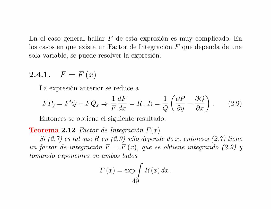
2.4. Factor de Integración: ODEs reducibles a Exactas. . . . . 462.4.1. F = F (x) . . . . . . . . . . . . . . . . . . . . . . 492.4.2. F
⇤= F
⇤(y) . . . . . . . . . . . . . . . . . . . . . 50
2.5. EDOs lineales . . . . . . . . . . . . . . . . . . . . . . . . 532.5.1. EDO lineal homogénea . . . . . . . . . . . . . . . 552.5.2. EDO lineal no homogénea . . . . . . . . . . . . . 56
2.6. ODE de Bernoulli: Reducción a una ODE Lineal . . . . . 63
iii

Parte I
Ecuaciones DiferencialesOrdinarias
1
Lección 1
Conceptos básicos
2
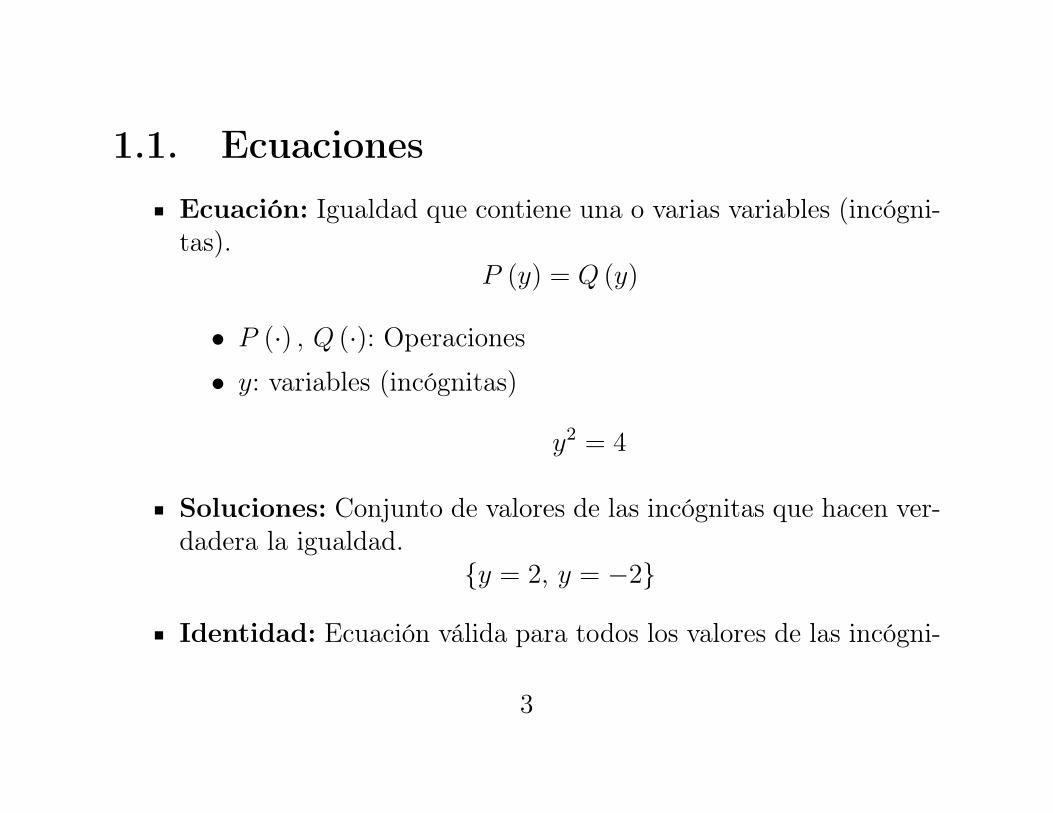
1.1. EcuacionesEcuación: Igualdad que contiene una o varias variables (incógni-tas).
P (y) = Q (y)
• P (·) , Q (·): Operaciones
• y: variables (incógnitas)
y
2= 4
Soluciones: Conjunto de valores de las incógnitas que hacen ver-dadera la igualdad.
{y = 2, y = �2}
Identidad: Ecuación válida para todos los valores de las incógni-
3
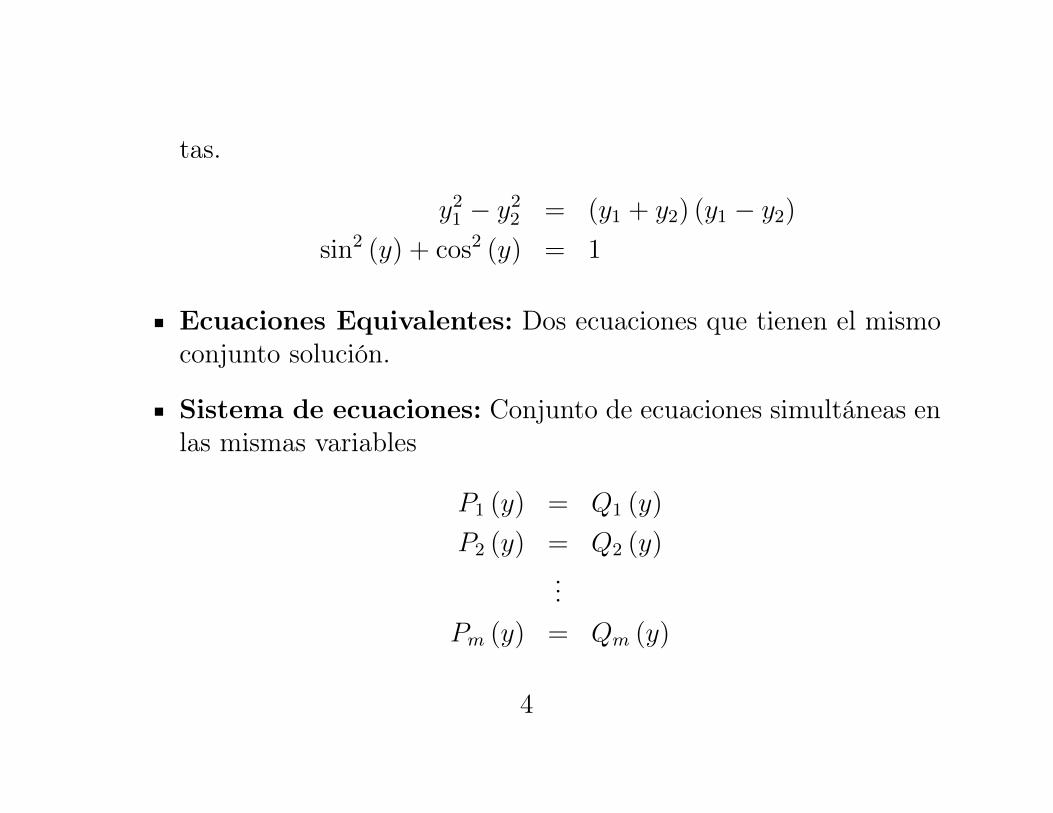
tas.
y
21 � y
22 = (y1 + y2) (y1 � y2)
sin
2(y) + cos
2(y) = 1
Ecuaciones Equivalentes: Dos ecuaciones que tienen el mismoconjunto solución.
Sistema de ecuaciones: Conjunto de ecuaciones simultáneas enlas mismas variables
P1 (y) = Q1 (y)
P2 (y) = Q2 (y)
...P
m
(y) = Q
m
(y)
4

Ejemplo:
3y1 + 5y2 = 2
5y1 + 8y2 = 3
Soluciones: Conjunto de valores de las incógnitas que hacen ver-daderas a todas las igualdades.
{y1 = �1, y2 = 1}
1.1.1. Tipos de Ecuaciones
Clasificación de acuerdo a los tipos de Operaciones (P (·) , Q (·)) yal tipo de Variables y
Univariables o Multivariables: una o múltiples variables.
5
• Ejemplo Univariable:
y
5 � 3y + 1 = 0
• Ejemplo Multivariable
y
41 +
1
2
y1y2 =1
3
y
32 � y
21y2 + y
22 �
1
7
Ecuaciones Algebráicas: Las Operaciones son polinomios y lasvariables son números complejos, reales, racionales. Se clasificande acuerdo al grado (máximo) de los polinomios
• Ecuaciones Lineales
3y1 + 5y2 = 2
5y1 + 8y2 = 3
6
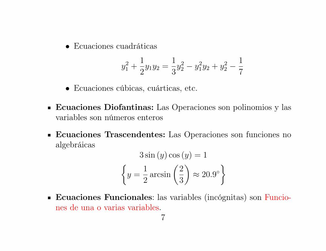
• Ecuaciones cuadráticas
y
21 +
1
2
y1y2 =1
3
y
22 � y
21y2 + y
22 �
1
7
• Ecuaciones cúbicas, cuárticas, etc.
Ecuaciones Diofantinas: Las Operaciones son polinomios y lasvariables son números enteros
Ecuaciones Trascendentes: Las Operaciones son funciones noalgebráicas
3 sin (y) cos (y) = 1
⇢y =
1
2
arcsin
✓2
3
◆⇡ 20.9
��
Ecuaciones Funcionales: las variables (incógnitas) son Funcio-nes de una o varias variables.
7
• Ecuaciones Diferenciales: Involucra derivadas de la (función)incógnita
• Ecuaciones Integrales: Involucra integrales de la (función) in-cógnita
• Ecuaciones Integro-diferenciales: Involucra derivadas e inte-grales de la (función) incógnita
1.1.2. Ecuaciones Diferenciales
Son Ecuaciones Funcionales que relacionan los valores de la funciónincógnita y sus derivadas. Son ecuaciones en las que aparecen las varia-bles independientes, la función incógnita y sus derivadas.
1.1.2.1. Ecuación Diferencial Ordinaria (EDO)
Incógnita: Función de una sola variable y : R ! R
8
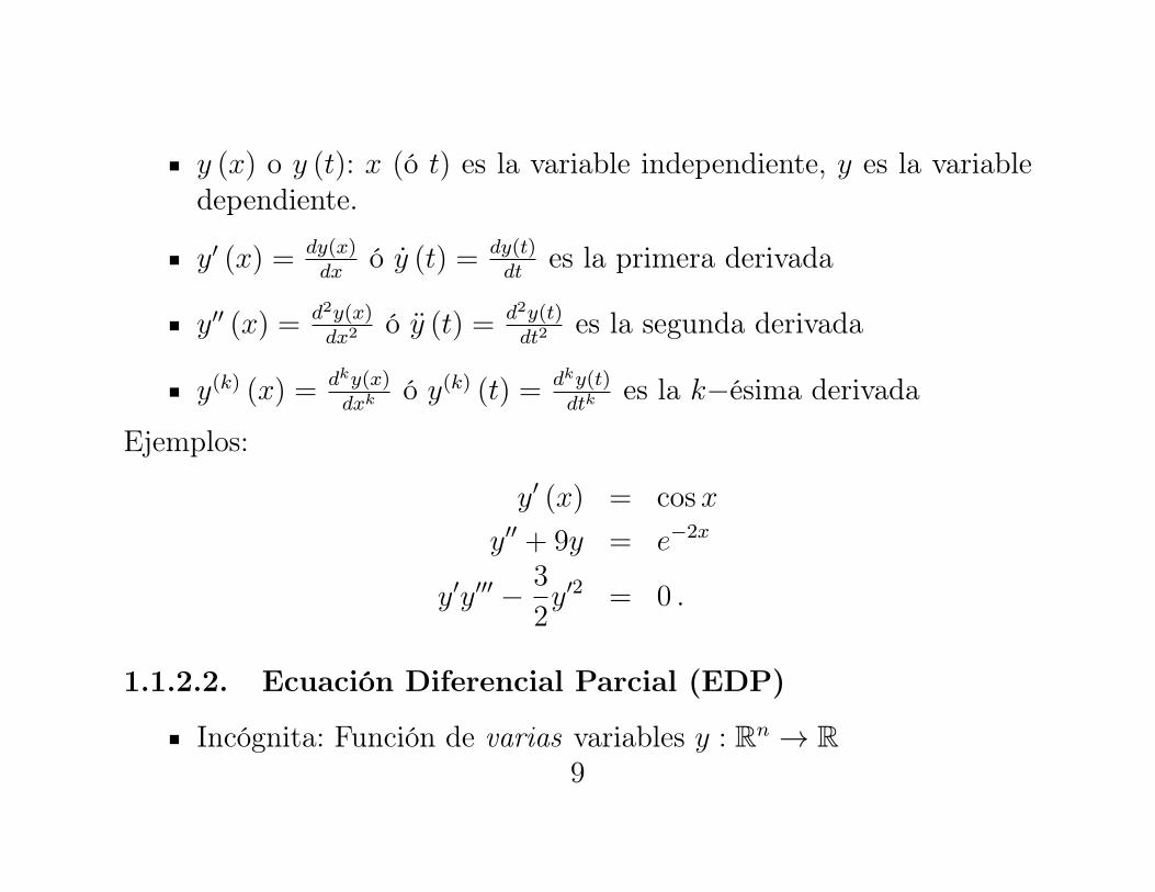
y (x) o y (t): x (ó t) es la variable independiente, y es la variabledependiente.
y
0(x) =
dy(x)dx
ó y (t) =
dy(t)dt
es la primera derivada
y
00(x) =
d
2y(x)dx
2 ó y (t) =
d
2y(t)dt
2 es la segunda derivada
y
(k)(x) =
d
ky(x)dx
k ó y
(k)(t) =
d
ky(t)dt
k es la k�ésima derivada
Ejemplos:
y
0(x) = cosx
y
00+ 9y = e
�2x
y
0y
000 � 3
2
y
02= 0 .
1.1.2.2. Ecuación Diferencial Parcial (EDP)
Incógnita: Función de varias variables y : Rn ! R9
• y (x): x = (x1, x2, · · · , xn
) son las variables independientes,y es la variable dependiente.
Ejemplo:@
2y (x)
@x
21
+
@
2y (x)
@x
22
= 0 .
1.2. Ecuaciones Diferenciales OrdinariasOrden de la EDO: Orden de la máxima derivada de la funciónincógnita que aparece en la ecuación. Una EDO es de orden n sila máxima derivada que aparece en la ecuación es y
(n)(x).
EDO Implícita: Si la ecuación no está resuelta con respecto a lamáxima derivada de la función incógnita.
EDO Explícita: Si la ecuación está resuelta con respecto a lamáxima derivada de la función incógnita.
10

1.2.1. EDO de Primer Orden
Ecuación Diferencial Ordinaria de Primer Orden en Forma Implícita:
F (x, y, y
0) = 0 .
Ejemplo:y
0
x
3� 4y
2= 0 .
Ecuación Diferencial Ordinaria de Primer Orden en Forma Explícita:
y
0= f (x, y) .
Ejemplo:y
0= 4x
3y
2.
11

1.2.2. EDO de Segundo Orden
Ecuación Diferencial Ordinaria de Segundo Orden en Forma Implí-cita:
F (x, y, y
0, y
00) = 0 .
Ecuación Diferencial Ordinaria de Segundo Orden en Forma Explí-cita:
y
00= f (x, y, y
0) .
Ejemplo: EDO de segundo orden lineal
y
00= f (x) y
0+ g (x) y + h (x) .
1.2.3. EDO de Orden n
Ecuación Diferencial Ordinaria de Orden nen Forma Implícita:
F
�x, y, y
0, · · · , y(n)
�= 0 .
12
Ecuación Diferencial Ordinaria de Orden n en Forma Explícita:
y
(n)= f
�x, y, y
0, · · · , y(n�1)
�.
1.2.4. Solución de una EDO
Una funcióny = h (x)
es una solución (o integral) de la EDO
F (x, y, y
0) = 0
en el intervalo abierto a < x < b (incluye los casos a = �1, b = 1) si
h (x) está definida y es diferenciable en el intervalo a < x < b, y
la ecuación se convierte en una identidad si se reemplazan y, y
0
por h, h
0 (respectivamente), es decir,
F (x, h (x) , h
0(x)) ⌘ 0 , 8x 2 (a, b) .
13

El grafo de h (x) se denomina también la Curva Solución o la CurvaIntegral de la EDO
Ejemplo 1.1 VerificaciónLa función y (x) = Ce
�x
2, para cualquier C 2 R, es solución en elintervalo x 2 (�1, 1) de la EDO
y
0+ 2xy = 0 .
Verificación: 8x 2 (�1, 1)
d
dx
⇣Ce
�x
2⌘+ 2x
⇣Ce
�x
2⌘= �2x
⇣Ce
�x
2⌘+ 2x
⇣Ce
�x
2⌘⌘ 0 .
ç
Ejemplo 1.2 Solución por cálculoLa familia de soluciones de la ODE
y
0= cosx ,
14
puede hallarse por integración de ambos ladosˆy
0dx =
ˆcos xdx+ c = sin x+ c ,
dónde c es una constante arbitraria (de integración).
Ejemplo 1.3 Crecimiento y Decrecimiento ExponencialesPor verificación se puede ver que una familia de soluciones de la
ODE linealy
0= ky ,
esy (x) = ce
kx
,
dónde c es una constante arbitraria.
Con k > 0 esta ecuación puede modelar crecimiento exponencial,como por ejemplo, una colonia de bacterias, población de animaleso de seres humanos (Ley de Malthus).
15

E X A M P L E 2 Solution by Calculus. Solution Curves
The ODE can be solved directly by integration on both sides. Indeed, using calculus,we obtain where c is an arbitrary constant. This is a family of solutions. Each valueof c, for instance, 2.75 or 0 or gives one of these curves. Figure 3 shows some of them, for
!!1, 0, 1, 2, 3, 4.c " !3, !2,!8,
y " !cos x dx " sin x # c,yr " dy>dx " cos x
SEC. 1.1 Basic Concepts. Modeling 5
y
x0
–4
2ππ–π
4
2
–2
Fig. 3. Solutions of the ODE yr " cos xy " sin x # c
0
0.5
1.0
1.5
2.5
2.0
0 2 4 6 8 10 12 14 t
y
Fig. 4B. Solutions of in Example 3 (exponential decay)
yr " !0.2y
0
10
20
30
40
0 2 4 6 8 10 12 14 t
y
Fig. 4A. Solutions of in Example 3 (exponential growth)
yr " 0.2y
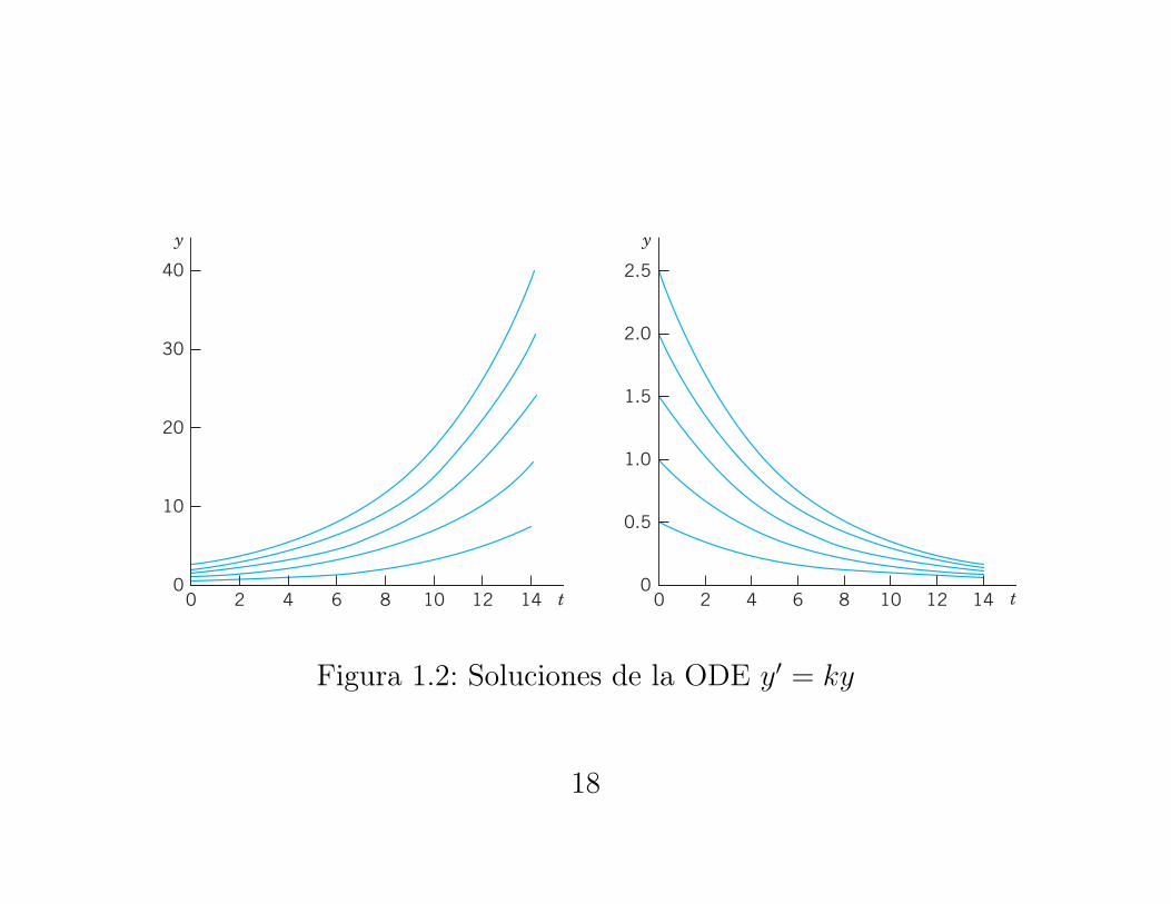
E X A M P L E 3 (A) Exponential Growth. (B) Exponential Decay
From calculus we know that has the derivative
Hence y is a solution of (Fig. 4A). This ODE is of the form With positive-constant k it canmodel exponential growth, for instance, of colonies of bacteria or populations of animals. It also applies tohumans for small populations in a large country (e.g., the United States in early times) and is then known asMalthus’s law.1 We shall say more about this topic in Sec. 1.5.
(B) Similarly, (with a minus on the right) has the solution (Fig. 4B) modelingexponential decay, as, for instance, of a radioactive substance (see Example 5). !
y " ce!0.2t,yr " !0.2
yr " ky.yr " 0.2y
yr "dy
dt" 0.2e0.2t " 0.2y.
y " ce0.2t
1Named after the English pioneer in classic economics, THOMAS ROBERT MALTHUS (1766–1834).
c01.qxd 7/30/10 8:14 PM Page 5
Figura 1.1: Soluciones de la ODE y
0= cosx
16
Con k < 0 esta ecuación puede modelar decrecimiento exponen-cial, como por ejemplo, una sustancia radioactiva.
Una funcióny = h (x)
es una solución (o integral) de la EDO de orden n
F
�x, y, y
0, · · · , y(n)
�= 0
en el intervalo abierto a < x < b (incluye los casos a = �1, b = 1) si
h (x) está definida y es n veces diferenciable en el intervalo a <
x < b, y
la ecuación se convierte en una identidad si se reemplazan y, y
0, · · · , y(n)
por h, h
0, · · · , h(n) (respectivamente), es decir,
F
�x, h (x) , h
0(x) , · · · , h(n)
(x)
�⌘ 0 , 8x 2 (a, b) .
17
E X A M P L E 2 Solution by Calculus. Solution Curves
The ODE can be solved directly by integration on both sides. Indeed, using calculus,we obtain where c is an arbitrary constant. This is a family of solutions. Each valueof c, for instance, 2.75 or 0 or gives one of these curves. Figure 3 shows some of them, for
!!1, 0, 1, 2, 3, 4.c " !3, !2,!8,
y " !cos x dx " sin x # c,yr " dy>dx " cos x
SEC. 1.1 Basic Concepts. Modeling 5
y
x0
–4
2ππ–π
4
2
–2
Fig. 3. Solutions of the ODE yr " cos xy " sin x # c
0
0.5
1.0
1.5
2.5
2.0
0 2 4 6 8 10 12 14 t
y
Fig. 4B. Solutions of in Example 3 (exponential decay)
yr " !0.2y
0
10
20
30
40
0 2 4 6 8 10 12 14 t
y
Fig. 4A. Solutions of in Example 3 (exponential growth)
yr " 0.2y
E X A M P L E 3 (A) Exponential Growth. (B) Exponential Decay
From calculus we know that has the derivative
Hence y is a solution of (Fig. 4A). This ODE is of the form With positive-constant k it canmodel exponential growth, for instance, of colonies of bacteria or populations of animals. It also applies tohumans for small populations in a large country (e.g., the United States in early times) and is then known asMalthus’s law.1 We shall say more about this topic in Sec. 1.5.
(B) Similarly, (with a minus on the right) has the solution (Fig. 4B) modelingexponential decay, as, for instance, of a radioactive substance (see Example 5). !
y " ce!0.2t,yr " !0.2
yr " ky.yr " 0.2y
yr "dy
dt" 0.2e0.2t " 0.2y.
y " ce0.2t
1Named after the English pioneer in classic economics, THOMAS ROBERT MALTHUS (1766–1834).
c01.qxd 7/30/10 8:14 PM Page 5
Figura 1.2: Soluciones de la ODE y
0= ky
18
1.2.5. Solución General y Particular de una EDO
La solución general o solución completa de una EDO de primer ordenes una función
y = h (x, C) ,
que depende de un parámetro real C, tal que para cualquier valor delparámetro (en un conjunto C 2 M), h (x, C) es una solución (o integral)de la EDO
F (x, y, y
0) = 0 .
Si se especifica un valor de la constante C se obtiene una soluciónparticular (sin constantes arbitrarias).
La solución general o solución completa de una EDO de orden n esuna función
y = h (x, C1, · · · , Cn
) ,
que depende de n parámetros reales (C1, · · · , Cn
), tal que para cualquiervalor del parámetro (en un conjunto (C1, · · · , Cn
) 2 M), h (x, C1, · · · , Cn
)
19

es una solución (o integral) de la EDO
F
�x, y, y
0, · · · , y(n)
�= 0 .
Si se especifica un valor de la constante C se obtiene una soluciónparticular (sin constantes arbitrarias).
Solución Singular: Son soluciones particulares de una EDO que nose pueden obtener de la solución general
Ejemplo 1.4 Solución singularLa ODE
(y
0)
2 � xy
0+ y = 0 ,
tiene como solución general (verificar por substitución)
y (x) = cx� c
2,
dónde c es una constante arbitraria.20

8 CHAP. 1 First-Order ODEs
1–8 CALCULUSSolve the ODE by integration or by remembering adifferentiation formula.1.2.3.4.5.6.7.8.
9–15 VERIFICATION. INITIAL VALUE PROBLEM (IVP)(a) Verify that y is a solution of the ODE. (b) Determinefrom y the particular solution of the IVP. (c) Graph thesolution of the IVP.9.
10.11.12.
13.
14.15. Find two constant solutions of the ODE in Prob. 13 by
inspection.16. Singular solution. An ODE may sometimes have an
additional solution that cannot be obtained from thegeneral solution and is then called a singular solution.The ODE is of this kind. Showby differentiation and substitution that it has thegeneral solution and the singular solution
. Explain Fig. 6.y ! x2>4 y ! cx " c2
yr2 " xyr # y ! 0
yr tan x ! 2y " 8, y ! c sin2 x # 4, y(12 p) ! 0
yr ! y " y2, y !1
1 # ce!x , y(0) ! 0.25
yyr ! 4x, y2 " 4x2 ! c (y $ 0), y(1) ! 4yr ! y # ex, y ! (x # c)ex, y(0) ! 1
2
yr # 5xy ! 0, y ! ce!2.5x2
, y(0) ! p
yr # 4y ! 1.4, y ! ce!4x # 0.35, y(0) ! 2
yt ! e!0.2xyr ! cosh 5.13xys ! "yyr ! 4e!x cos xyr ! "1.5yyr ! yyr # xe!x2>2 ! 0yr # 2 sin 2px ! 0
17–20 MODELING, APPLICATIONSThese problems will give you a first impression of modeling.Many more problems on modeling follow throughout thischapter.
17. Half-life. The half-life measures exponential decay.It is the time in which half of the given amount ofradioactive substance will disappear. What is the half-life of (in years) in Example 5?
18. Half-life. Radium has a half-life of about3.6 days.(a) Given 1 gram, how much will still be present after1 day?(b) After 1 year?
19. Free fall. In dropping a stone or an iron ball, airresistance is practically negligible. Experimentsshow that the acceleration of the motion is constant(equal to called theacceleration of gravity). Model this as an ODE for
, the distance fallen as a function of time t. If themotion starts at time from rest (i.e., with velocity
), show that you obtain the familiar law offree fall
20. Exponential decay. Subsonic flight. The efficiencyof the engines of subsonic airplanes depends on airpressure and is usually maximum near ft.Find the air pressure at this height. Physicalinformation. The rate of change is proportionalto the pressure. At ft it is half its value
at sea level. Hint. Remember from calculusthat if then Can you seewithout calculation that the answer should be closeto ?y0>4 yr ! kekx ! ky.y ! ekx,y0 ! y(0)
18,000yr(x)
y(x)35,000
y ! 12 gt 2.
v ! yr ! 0t ! 0
y(t)
g ! 9.80 m>sec2 ! 32 ft>sec2,
22488 Ra
22688
Ra
P R O B L E M S E T 1 . 1
–4 42
y
x
21
3
–4–5
–2–3
–2–1
Fig. 6. Particular solutions and singular solution in Problem 16
c01.qxd 7/30/10 8:15 PM Page 8
Figura 1.3: Soluciones particulares y solución singular de la ODE (y
0)
2�xy
0+ y = 0 .
Solución singular
y (x) =
x
2
4
.
21
1.3. Ecuaciones Diferenciales de Primer Or-den
Considere la EDO de primer orden en forma explícita
y
0= f (x, y) .
La solución general contiene una constante arbitraria C.
1.3.1. Problema de valores (o condiciones) iniciales:PCI
Una forma de especificar la solución particular es mediante una con-dición inicial (C.I.), es decir,
y (x0) = y0 ,
con valores dados x0 e y0.22

Un problema de valores iniciales es:
Una ODE (explícita por ejemplo): y0 = f (x, y) ,
Una condición inicial: y (x0) = y0 .
Ejemplo 1.5 Crecimiento y Decrecimiento ExponencialesResuelva el problem de valores iniciales
y
0= 3y , y (0) = 5.7 .
La solución general esy (x) = ce
3x.
De la solución general y la condición inicial se obtiene
y (0) = ce
0= c = 5.7 .
Así que la (única) solución del problema de valores iniciales es: y (x) =5.7e
3x.23
1.3.2. Interpretación Geométrica y gráfica
Del cálculo: y0 (x) es la pendiente de y (x). ) Curva solución de
y
0= f (x, y)
que pasa por el punto (x0, y0) debe tener en ese punto la pendientey
0(x0) igual al valor de f en ese punto, es decir,
y
0(x0) = f (x0, y0) .
Podemos mostrar las direcciones de las curvas solución de una EDOdibujando pequeños segmentos de recta en el plano xy. Esto representael campo de direcciones (o campo de pendientes), en el que se puedenajustar (aproximar) curvas solución. Esto puede revelar propiedades tí-picas de la familia de soluciones (ver Figura 1.4).
24

1.2 Geometric Meaning of Direction Fields, Euler’s Method
A first-order ODE
(1)
has a simple geometric interpretation. From calculus you know that the derivative ofis the slope of . Hence a solution curve of (1) that passes through a point
must have, at that point, the slope equal to the value of f at that point; that is,
Using this fact, we can develop graphic or numeric methods for obtaining approximatesolutions of ODEs (1). This will lead to a better conceptual understanding of an ODE (1).Moreover, such methods are of practical importance since many ODEs have complicatedsolution formulas or no solution formulas at all, whereby numeric methods are needed.
Graphic Method of Direction Fields. Practical Example Illustrated in Fig. 7. Wecan show directions of solution curves of a given ODE (1) by drawing short straight-linesegments (lineal elements) in the xy-plane. This gives a direction field (or slope field)into which you can then fit (approximate) solution curves. This may reveal typicalproperties of the whole family of solutions.
Figure 7 shows a direction field for the ODE
(2)
obtained by a CAS (Computer Algebra System) and some approximate solution curvesfitted in.
yr ! y " x
yr(x0) ! f (x0, y0).
yr(x0)(x0, y0)y(x)y(x)yr(x)
yr ! f (x, y)
yr ! f (x, y).
SEC. 1.2 Geometric Meaning of y# ! ƒ(x, y). Direction Fields, Euler’s Method 9
1
2
0.5 1–0.5–1–1.5–2
–1
–2
y
x
Fig. 7. Direction field of with three approximate solution curves passing through (0, 1), (0, 0), (0, ), respectively$1
yr ! y " x,
c01.qxd 7/30/10 8:15 PM Page 9
Figura 1.4: Campo de direcciones de y
0= y + x , con tres soluciones
aproximadas que pasan por (0, 1) , (0, 0) , (0, �1).
25
Lección 2
Métodos de solución de EDOsde Primer Orden
Veremos algunos tipos de EDOs que se pueden resolver fácilmente:
26
EDOs Separables y EDOs reducibles a separables.
EDOs Exactas y Factores de Integración
EDOs lineales, Ecuación de Bernoulli
2.1. EDOs Separables: Método de Separa-ción de Variables.
Considere una EDO que se pueda escribir de la forma
g (y) y
0= f (x) .
Integrando a ambos lados con respecto a x se obtieneˆ
g (y)
✓dy
dx
◆dx =
ˆf (x) dx+ C ,
27
que se puede escribir´g (y) dy =
´f (x) dx+ C .
Evaluando las integrales obtenemos una solución general de la EDO.Método de Separación de Variables, ya que el lado izquierdo solo de-pende de y y el lado derecho solo de x.
Ejemplo 2.1 EDO separableLa EDO
y
0= 1 + y
2
es separable, porque puede ser escrita como
dy
1 + y
2= dx )
ˆdy
1 + y
2=
ˆdx+C ) arctan y = x+C , y = tan (x+ C) .
28

Comentario 2.2Es muy importante introducir la constante de in-tegración inmediatamente después de realizar laintegración!
Si se realiza de la siguiente manera el resultado es incorrecto!
dy
1 + y
2= dx )
ˆdy
1 + y
2=
ˆdx ) arctan y = x ) y = tan x+ C .
Ejemplo 2.3 EDO separableLa EDO
y
0= (x+ 1) e
�x
y
2
es separable, porque puede ser escrita como
dy
y
2= (x+ 1) e
�x
dx )ˆ
dy
y
2=
ˆ(x+ 1) e
�x
dx+ C )
) �1
y
= � (x+ 2) e
�x
+ C , y =
1
(x+ 2) e
�x � C
.
29
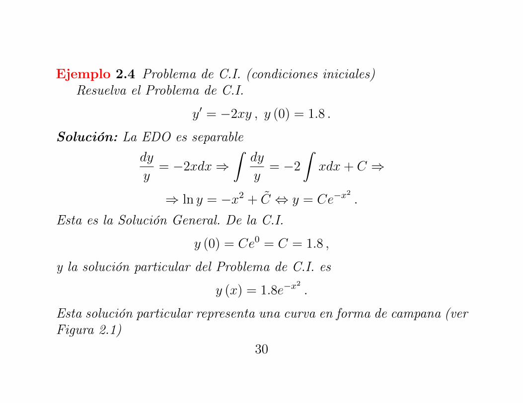
Ejemplo 2.4 Problema de C.I. (condiciones iniciales)Resuelva el Problema de C.I.
y
0= �2xy , y (0) = 1.8 .
Solución: La EDO es separabledy
y
= �2xdx )ˆ
dy
y
= �2
ˆxdx+ C )
) ln y = �x
2+
˜
C , y = Ce
�x
2.
Esta es la Solución General. De la C.I.
y (0) = Ce
0= C = 1.8 ,
y la solución particular del Problema de C.I. es
y (x) = 1.8e
�x
2.
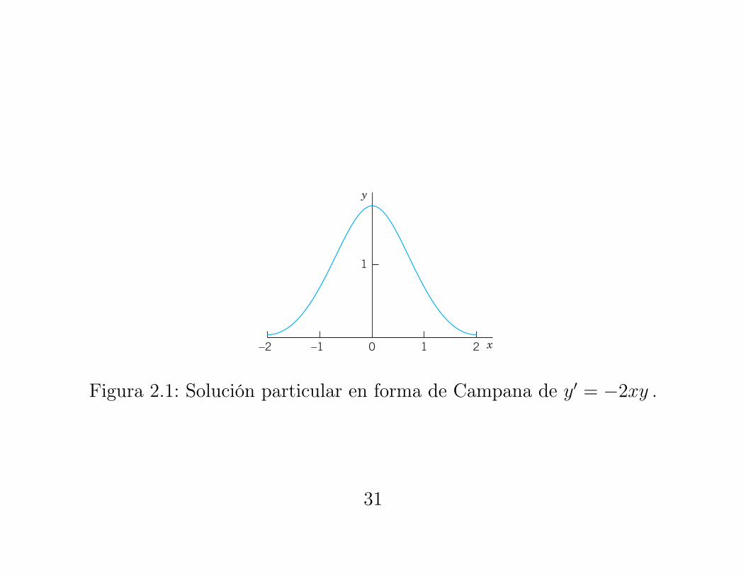
Esta solución particular representa una curva en forma de campana (verFigura 2.1)
30
E X A M P L E 2 Separable ODE
The ODE is separable; we obtain
E X A M P L E 3 Initial Value Problem (IVP). Bell-Shaped Curve
Solve
Solution. By separation and integration,
This is the general solution. From it and the initial condition, Hence the IVP has thesolution This is a particular solution, representing a bell-shaped curve (Fig. 10). !y ! 1.8e!x2
.y(0) ! ce0 ! c ! 1.8.
dy
y! "2x dx, ln y ! "x2 # c!, y ! ce!x2
.
yr ! "2xy, y(0) ! 1.8.
!By integration, "y!1 ! "(x # 2)e!x # c, y !
1(x # 2)e"x " c
.
y!2 dy ! (x # 1)e!x dx.yr ! (x # 1)e!xy2
SEC. 1.3 Separable ODEs. Modeling 13
1
10–1–2 2 x
y
Fig. 10. Solution in Example 3 (bell-shaped curve)
ModelingThe importance of modeling was emphasized in Sec. 1.1, and separable equations yieldvarious useful models. Let us discuss this in terms of some typical examples.
E X A M P L E 4 Radiocarbon Dating2
In September 1991 the famous Iceman (Oetzi), a mummy from the Neolithic period of the Stone Age found inthe ice of the Oetztal Alps (hence the name “Oetzi”) in Southern Tyrolia near the Austrian–Italian border, causeda scientific sensation. When did Oetzi approximately live and die if the ratio of carbon to carbon inthis mummy is 52.5% of that of a living organism?
Physical Information. In the atmosphere and in living organisms, the ratio of radioactive carbon (maderadioactive by cosmic rays) to ordinary carbon is constant. When an organism dies, its absorption of by breathing and eating terminates. Hence one can estimate the age of a fossil by comparing the radioactivecarbon ratio in the fossil with that in the atmosphere. To do this, one needs to know the half-life of , whichis 5715 years (CRC Handbook of Chemistry and Physics, 83rd ed., Boca Raton: CRC Press, 2002, page 11–52,line 9).
Solution. Modeling. Radioactive decay is governed by the ODE (see Sec. 1.1, Example 5). Byseparation and integration (where t is time and is the initial ratio of to )
(y0 ! ec).y ! y0 ektln ƒ y ƒ ! kt # c,
dy
y! k dt,
126 C14
6 Cy0
yr ! ky
146 C
146 C12
6 C
146 C
126 C14
6 C
2Method by WILLARD FRANK LIBBY (1908–1980), American chemist, who was awarded for this workthe 1960 Nobel Prize in chemistry.
c01.qxd 7/30/10 8:15 PM Page 13
Figura 2.1: Solución particular en forma de Campana de y
0= �2xy .
31

2.2. EDOs reducibles a EDOs SeparablesAlgunas EDOs pueden ser reducidas a separables mediante una trans-
formación de la variable y.
2.2.1. EDOs “homogéneas”
Sea una EDO del tipo
y
0= f
�y
x
�.
f es una función contínua de y
x
. La transformación
u (x) =
y (x)
x
) y (x) = u (x) x ) y
0= u
0x+ u .
Substituyendo en la EDO se obtiene
u
0x+ u = f (u) ) u
0x = f (u)� u .
32
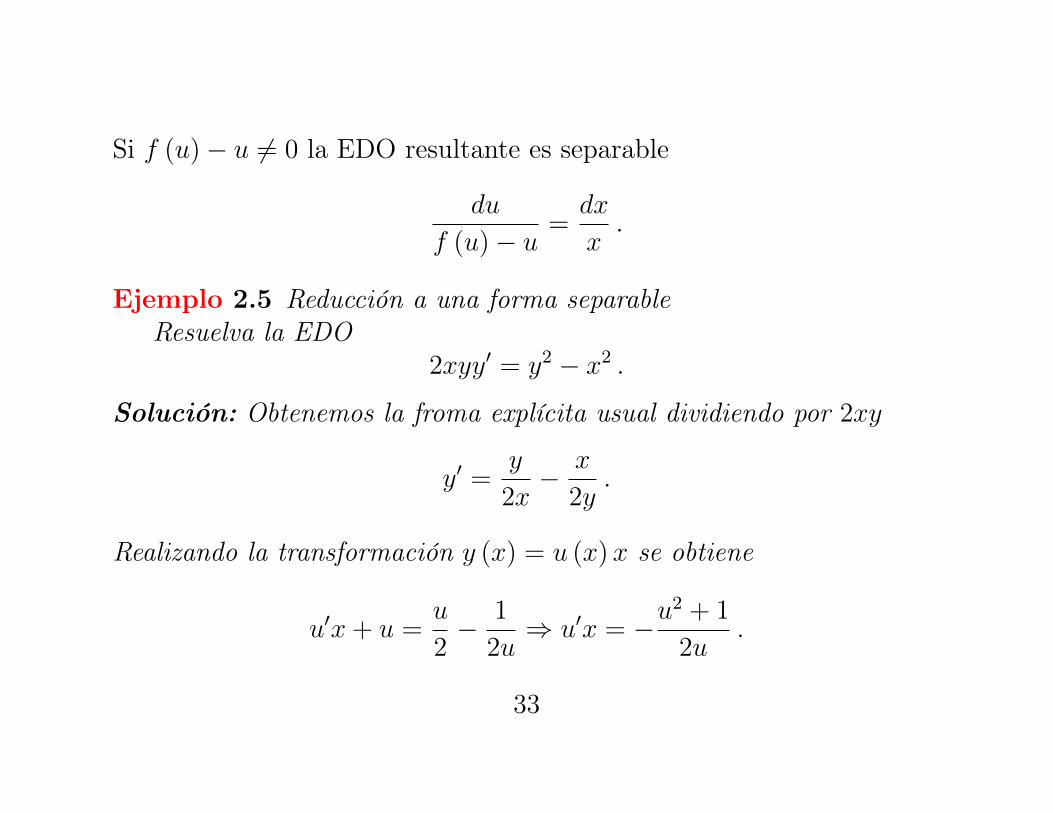
Si f (u)� u 6= 0 la EDO resultante es separable
du
f (u)� u
=
dx
x
.
Ejemplo 2.5 Reducción a una forma separableResuelva la EDO
2xyy
0= y
2 � x
2.
Solución: Obtenemos la froma explícita usual dividiendo por 2xy
y
0=
y
2x
� x
2y
.
Realizando la transformación y (x) = u (x) x se obtiene
u
0x+ u =
u
2
� 1
2u
) u
0x = �u
2+ 1
2u
.
33

Esta EDO es de variables separables2u
u
2+ 1
du = �dx
x
)ˆ
2u
u
2+ 1
du = �ˆ
dx
x
+ C )
) ln
�1 + u
2�= � ln |x|+ ˜
C ) ln
�1 + u
2�= ln
1
|x| +˜
C .
Tomando exponenciales en ambos lados se obtiene
1+u
2=
C
x
, 1+
⇣y
x
⌘2
=
C
x
) x
2+y
2= Cx )
✓x� C
2
◆2
+y
2=
C
2
4
.
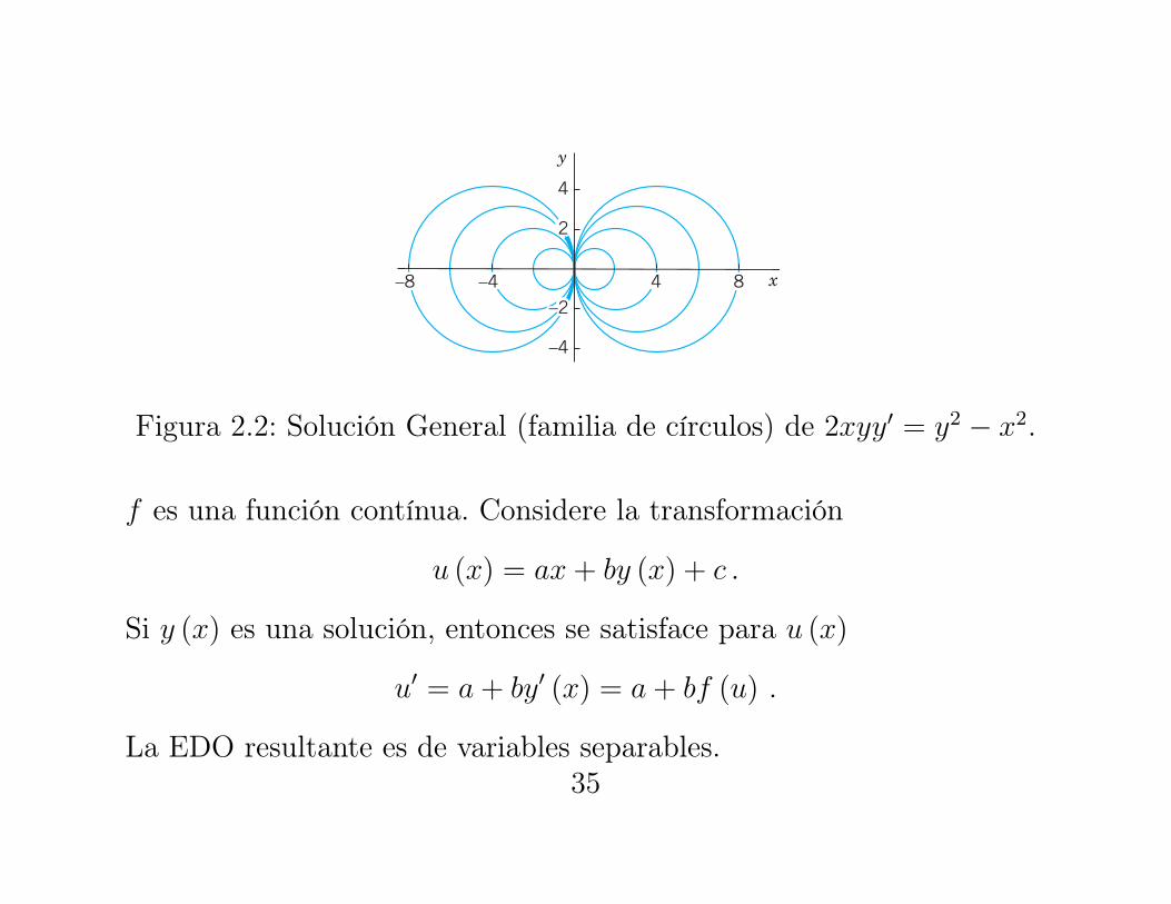
Esta es la Solución General de la EDO y representa una familia decírculos que pasan por el origen, con centros en el eje x (ver Figura 2.2)
2.2.2. Otra EDO reducible a separable
Sea una EDO del tipo
y
0= f (ax+ by + c) , b 6= 0 .
34
E X A M P L E 8 Reduction to Separable Form
Solve
Solution. To get the usual explicit form, divide the given equation by 2xy,
Now substitute y and from (9) and then simplify by subtracting u on both sides,
You see that in the last equation you can now separate the variables,
By integration,
Take exponents on both sides to get or . Multiply the last equation by toobtain (Fig. 14)
Thus
This general solution represents a family of circles passing through the origin with centers on the x-axis. !
ax !c2b2 " y2 #
c2
4.x2 " y2 # cx.
x21 " (y>x)2 # c>x1 " u2 # c>xln (1 " u2) # !ln ƒ x ƒ " c* # ln ` 1
x` " c*.
2u du
1 " u2# !
dxx
.
urx # !u2
!12u
#!u2 ! 1
2u.urx " u #
u2
!1
2u,
yr
yr #y2 ! x2
2xy#
y
2x!
x2y
.
2xyyr # y2 ! x2.
18 CHAP. 1 First-Order ODEs
4
–4
y
x–4–8 4 8
2
–2
Fig. 14. General solution (family of circles) in Example 8
1. CAUTION! Constant of integration. Why is itimportant to introduce the constant of integrationimmediately when you integrate?
2–10 GENERAL SOLUTIONFind a general solution. Show the steps of derivation. Checkyour answer by substitution.2.3.4.5.6.
7.
8.9.
10. xyr # x " y (Set y>x # u)xyr # y2 " y (Set y>x # u)yr # (y " 4x)2 (Set y " 4x # v)
xyr # y " 2x3 sin2 y
x (Set y>x # u)
yr # e2x!1y2
yyr " 36x # 0yr sin 2px # py cos 2pxyr # sec2 yy3yr " x3 # 0
11–17 INITIAL VALUE PROBLEMS (IVPS)Solve the IVP. Show the steps of derivation, beginning withthe general solution.
11.
12.
13.
14.
15.
16.(Set )
17.
18. Particular solution. Introduce limits of integration in(3) such that y obtained from (3) satisfies the initialcondition y(x0) # y0.
(Set y>x # u)xyr # y " 3x4 cos2 (y>x), y(1) # 0
v # x " y ! 2yr # (x " y ! 2)2, y(0) # 2
yr # !4x>y, y(2) # 3
dr>dt # !2tr, r(0) # r0
yrcosh2 x # sin2 y, y(0) # 12 p
yr # 1 " 4y2, y(1) # 0
xyr " y # 0, y(4) # 6
P R O B L E M S E T 1 . 3
c01.qxd 7/30/10 8:15 PM Page 18
Figura 2.2: Solución General (familia de círculos) de 2xyy
0= y
2 � x
2.
f es una función contínua. Considere la transformación
u (x) = ax+ by (x) + c .
Si y (x) es una solución, entonces se satisface para u (x)
u
0= a+ by
0(x) = a+ bf (u) .
La EDO resultante es de variables separables.35
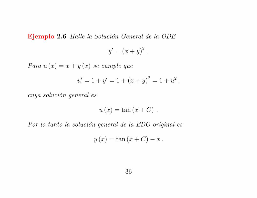
Ejemplo 2.6 Halle la Solución General de la ODE
y
0= (x+ y)
2.
Para u (x) = x+ y (x) se cumple que
u
0= 1 + y
0= 1 + (x+ y)
2= 1 + u
2,
cuya solución general es
u (x) = tan (x+ C) .
Por lo tanto la solución general de la EDO original es
y (x) = tan (x+ C)� x .
36
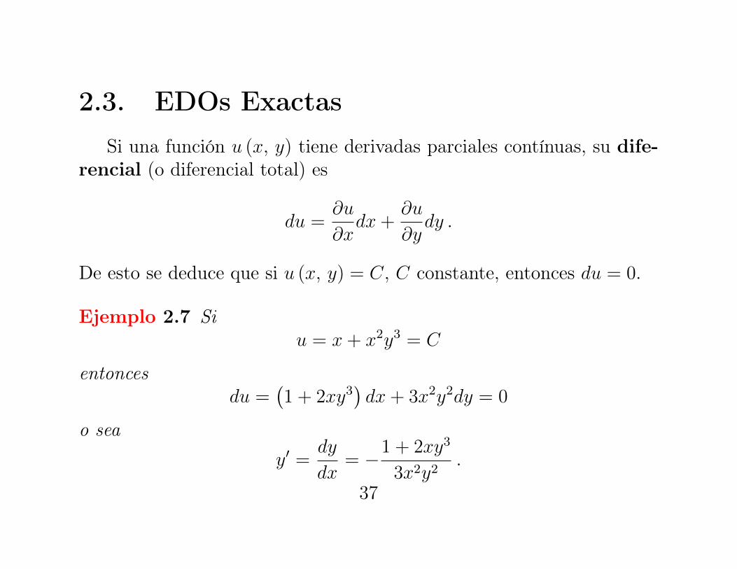
2.3. EDOs ExactasSi una función u (x, y) tiene derivadas parciales contínuas, su dife-
rencial (o diferencial total) es
du =
@u
@x
dx+
@u
@y
dy .
De esto se deduce que si u (x, y) = C, C constante, entonces du = 0.
Ejemplo 2.7 Siu = x+ x
2y
3= C
entoncesdu =
�1 + 2xy
3�dx+ 3x
2y
2dy = 0
o seay
0=
dy
dx
= �1 + 2xy
3
3x
2y
2.
37
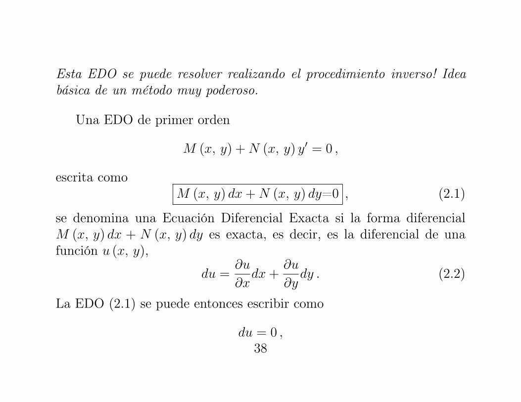
Esta EDO se puede resolver realizando el procedimiento inverso! Ideabásica de un método muy poderoso.
Una EDO de primer orden
M (x, y) +N (x, y) y
0= 0 ,
escrita comoM (x, y) dx+N (x, y) dy=0 , (2.1)
se denomina una Ecuación Diferencial Exacta si la forma diferencialM (x, y) dx + N (x, y) dy es exacta, es decir, es la diferencial de unafunción u (x, y),
du =
@u
@x
dx+
@u
@y
dy . (2.2)
La EDO (2.1) se puede entonces escribir como
du = 0 ,
38
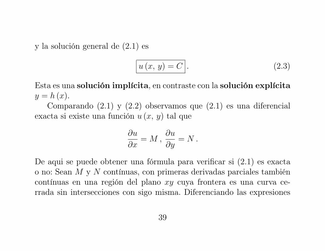
y la solución general de (2.1) es
u (x, y) = C . (2.3)
Esta es una solución implícita, en contraste con la solución explícitay = h (x).
Comparando (2.1) y (2.2) observamos que (2.1) es una diferencialexacta si existe una función u (x, y) tal que
@u
@x
= M ,
@u
@y
= N .
De aqui se puede obtener una fórmula para verificar si (2.1) es exactao no: Sean M y N contínuas, con primeras derivadas parciales tambiéncontínuas en una región del plano xy cuya frontera es una curva ce-rrada sin intersecciones con sigo misma. Diferenciando las expresiones
39

anteriores se obtiene@
2u
@y@x
=
@M
@y
,
@
2u
@x@y
=
@N
@x
.
Por la hipótesis de continuidad de las dos derivadas parciales de segundoorden, deben ser iguales, y por lo tanto
@M
@y
=
@N
@x
. (2.4)
Esta condición es necesaria y suficiente para que (2.1) sea una EcuaciónDiferencial Exacta.
Si (2.1) es Exacta, la función u (x, y) puede obtenerse por inspeccióno de la siguiente forma sistemática
De @u
@x
= M se obtiene mediante integración con respecto a x
u =
´Mdx+ k (y) . (2.5)40

En la integración, yse toma como constante, y k (y) juega el papelde una “constante” de integración. Para determinar k (y), obtene-mos @u
@y
de (2.5), usamos @u
@y
= N para obtener dk
dy
y lo integramospara obtener a k.
De @u
@y
= N se obtiene mediante integración con respecto a y
u =
´Ndy + l (x) . (2.6)
Para determinar l (x), obtenemos @u
@x
de (2.6), usamos @u
@x
= M
para obtener dl
dx
y lo integramos para obtener a l.
Ejemplo 2.8 EDO ExactaResuelva la EDO
cos (x+ y) dx+
�3y
2+ 2y + cos (x+ y)
�dy = 0 .
Solución: Paso 1. Verificación de exactitud.
41
Ecuación de la forma (2.1) con
M = cos (x+ y) , N = 3y
2+ 2y + cos (x+ y) .
Por lo tanto, la condición de exactitud (2.4)@M
@y
= � sin (x+ y) =
@N
@x
= � sin (x+ y)
se satisface.Paso 2. Solución General Implícita. De (2.5) obtenemos me-
diante integración
u =
ˆMdx+ k (y) =
ˆcos (x+ y) dx+ k (y) = sin (x+ y) + k (y) .
Para hallar k (y) diferenciamos esta expresión con respecto a y y usamosla fórmula @u
@y
= N , obteniendo
@u
@y
= cos (x+ y) +
dk (y)
dy
= N = 3y
2+ 2y + cos (x+ y) )
42
) dk (y)
dy
= 3y
2+ 2y ) k = y
3+ y
2+
˜
C .
Así obtenemos la solución general
u (x, y) = sin (x+ y) + y
3+ y
2= C .
Paso 3. Verificar la Solución General Implícita. Se puedeverificar mediante la diferenciación (implícita) de la solución implícitau (x, y) = C si se obtiene la EDO:
du =
@u
@x
dx+
@u
@y
dy = cos (x+ y) dx+
�cos (x+ y) + 3y
2+ 2y
�dy = dC = 0 .
Esto completa la verificación.
Ejemplo 2.9 Un problema de C.I.Resuelva el problema de C.I.
(cos y sinh x+ 1) dx� sin y cosh xdy = 0 , y (1) = 2 .
43
Solución: Se puede verificar que la EDO es exacta. Para encontrar au usamos (2.6)
u =
ˆNdy + l (x) = �
ˆsin y cosh xdy + l (x) = cos y cosh x+ l (x) .
Para hallar la l (x) usamos
@u
@x
= cos y sinh x+
dl (x)
dx
= M = cos y sinh x+ 1 )
) dl (x)
dx
= 1 ) l (x) = x+ C
⇤
entonces la solución general es
u (x, y) = cos y cosh x+ x = C .
De la C.I.u (1, 2) = cos 2 cosh 1 + 1 = 0.358 = C .
44

Step 3. Checking an implicit solution. We can check by differentiating the implicit solution implicitly and see whether this leads to the given ODE (7):
(9)
This completes the check.
E X A M P L E 2 An Initial Value Problem
Solve the initial value problem
(10)
Solution. You may verify that the given ODE is exact. We find u. For a change, let us use (6*),
From this, Hence By integration, This gives the general solution From the initial condition,
Hence the answer is cos y cosh Figure 17 shows the particular solutions for (thicker curve), 1, 2, 3. Check that the answer satisfies the ODE. (Proceed as in Example 1.) Also check that theinitial condition is satisfied. !
c ! 0, 0.358x " x ! 0.358.0.358 ! c.cos 2 cosh 1 " 1 !u(x, y) ! cos y cosh x " x ! c.
l(x) ! x " c*.dl>dx ! 1.0u>0x ! cos y sinh x " dl>dx ! M ! cos y sinh x " 1.
u ! #!sin y cosh x dy " l(x) ! cos y cosh x " l(x).
y(1) ! 2.(cos y sinh x " 1) dx # sin y cosh x dy ! 0,
!
du !0u0x
dx "0u0y
dy ! cos (x " y) dx " (cos (x " y) " 3y2 " 2y) dy ! 0.
u(x, y) ! c
SEC. 1.4 Exact ODEs. Integrating Factors 23
y
x0 1.0 2.0 3.00.5 1.5 2.5
1.0
2.0
0.5
1.5
2.5
Fig. 17. Particular solutions in Example 2
E X A M P L E 3 WARNING! Breakdown in the Case of Nonexactness
The equation is not exact because and so that in (5), butLet us show that in such a case the present method does not work. From (6),
hence
Now, should equal by (4b). However, this is impossible because can depend only on . Try(6*); it will also fail. Solve the equation by another method that we have discussed.
Reduction to Exact Form. Integrating FactorsThe ODE in Example 3 is It is not exact. However, if we multiply itby , we get an exact equation [check exactness by (5)!],
(11)
Integration of (11) then gives the general solution y>x ! c ! const.
#y dx " x dy
x2 ! #y
x2 dx "1x
dy ! d ayxb ! 0.
1>x2#y dx " x dy ! 0.
!yk(y)N ! x,0u>0y
0u0y
! #x "dkdy
.u ! !M dx " k(y) ! #xy " k(y),
0N>0x ! 1.0M>0y ! #1N ! x,M ! #y#y dx " x dy ! 0
c01.qxd 7/30/10 8:15 PM Page 23
Figura 2.3: Soluciones Particulares u (x, y) = cos y cosh x+ x = C paravalores de C = 0, 0.358, 1, 2, 3.
45

La solución particular es entonces u (x, y) = cos y cosh x+x = 0.358
(ver Figura 2.3)
2.4. Factor de Integración: ODEs reduciblesa Exactas.
Ejemplo 2.10 MotivaciónLa ODE
�ydx+ xdy = 0
no es exacta, ya que no se satisface (2.4):@M
@y
= �1 6= @N
@x
= 1 .
Si multiplicamos la EDO por 1/x
2 obtenemos la ODE exacta
� y
x
2dx+
1
x
dy = d
⇣y
x
⌘= 0 .
46

Por integración obtenemos la solución generaly
x
= C ,
C constante.
La idea derivada del ejemplo es: Multiplique una EDO no exacta
P (x, y) dx+Q (x, y) dy = 0 , (2.7)
por una función (en general de x e y) F (x, y) de tal forma que la EDOresultante
F (x, y)P (x, y) dx+ F (x, y)Q (x, y) dy = 0 (2.8)
sea exacta. F (x, y) is denominada Factor de Integración de (2.7).
Ejemplo 2.11 El factor de integración en el ejemplo 2.10 es F =
1/x
2.Es notable que uno puede encontrar otros factores de integración paraesta ecuación:
47
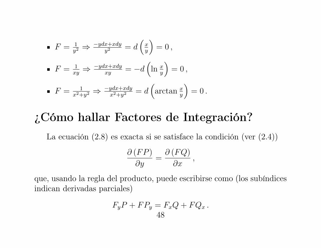
F =
1y
2 ) �ydx+xdy
y
2 = d
⇣x
y
⌘= 0 ,
F =
1xy
) �ydx+xdy
xy
= �d
⇣ln
x
y
⌘= 0 ,
F =
1x
2+y
2 ) �ydx+xdy
x
2+y
2 = d
⇣arctan
x
y
⌘= 0 .
¿Cómo hallar Factores de Integración?La ecuación (2.8) es exacta si se satisface la condición (ver (2.4))
@ (FP )
@y
=
@ (FQ)
@x
,
que, usando la regla del producto, puede escribirse como (los subíndicesindican derivadas parciales)
F
y
P + FP
y
= F
x
Q+ FQ
x
.
48
En el caso general hallar F de esta expresión es muy complicado. Enlos casos en que exista un Factor de Integración F que dependa de unasola variable, se puede resolver la expresión.
2.4.1. F = F (x)
La expresión anterior se reduce a
FP
y
= F
0Q+ FQ
x
) 1
F
dF
dx
= R , R =
1
Q
✓@P
@y
� @Q
@x
◆. (2.9)
Entonces se obtiene el siguiente resultado:
Teorema 2.12 Factor de Integración F (x)
Si (2.7) es tal que R en (2.9) sólo depende de x, entonces (2.7) tieneun factor de integración F = F (x), que se obtiene integrando (2.9) ytomando exponentes en ambos lados
F (x) = exp
ˆR (x) dx .
49
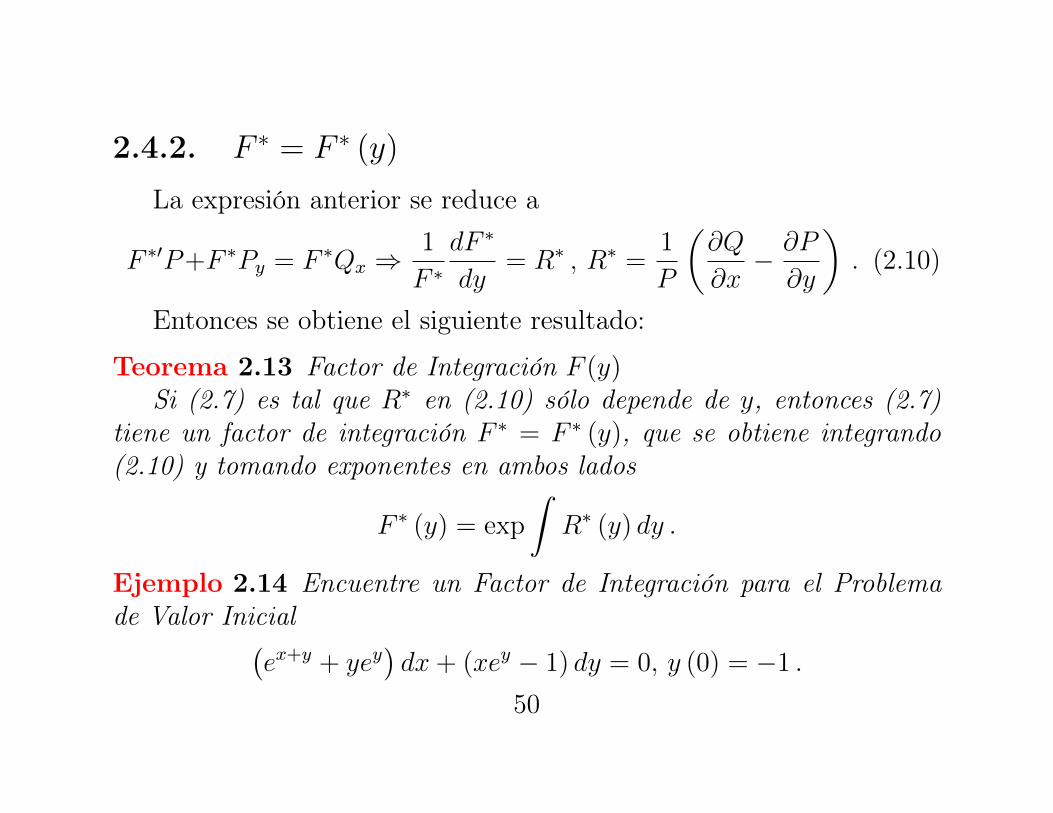
2.4.2. F
⇤= F
⇤(y)
La expresión anterior se reduce a
F
⇤0P+F
⇤P
y
= F
⇤Q
x
) 1
F
⇤dF
⇤
dy
= R
⇤, R
⇤=
1
P
✓@Q
@x
� @P
@y
◆. (2.10)
Entonces se obtiene el siguiente resultado:
Teorema 2.13 Factor de Integración F (y)
Si (2.7) es tal que R
⇤ en (2.10) sólo depende de y, entonces (2.7)tiene un factor de integración F
⇤= F
⇤(y), que se obtiene integrando
(2.10) y tomando exponentes en ambos lados
F
⇤(y) = exp
ˆR
⇤(y) dy .
Ejemplo 2.14 Encuentre un Factor de Integración para el Problemade Valor Inicial
�e
x+y
+ ye
y
�dx+ (xe
y � 1) dy = 0, y (0) = �1 .
50
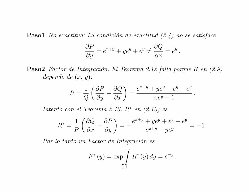
Paso1 No exactitud: La condición de exactitud (2.4) no se satisface
@P
@y
= e
x+y
+ ye
y
+ e
y 6= @Q
@x
= e
y
.
Paso2 Factor de Integración. El Teorema 2.12 falla porque R en (2.9)depende de (x, y):
R =
1
Q
✓@P
@y
� @Q
@x
◆=
e
x+y
+ ye
y
+ e
y � e
y
xe
y � 1
.
Intento con el Teorema 2.13. R⇤ en (2.10) es
R
⇤=
1
P
✓@Q
@x
� @P
@y
◆= �e
x+y
+ ye
y
+ e
y � e
y
e
x+y
+ ye
y
= �1 .
Por lo tanto un Factor de Integración es
F
⇤(y) = exp
ˆR
⇤(y) dy = e
�y
.
51
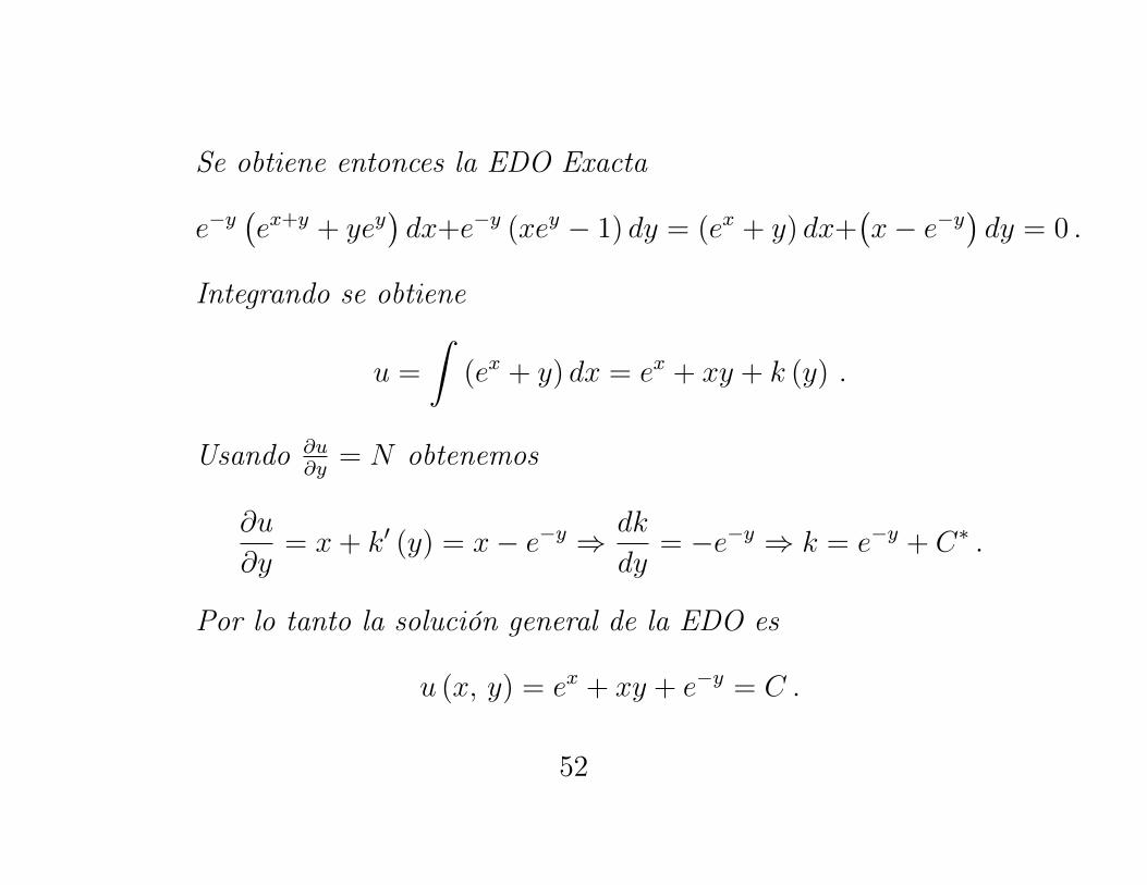
Se obtiene entonces la EDO Exacta
e
�y
�e
x+y
+ ye
y
�dx+e
�y
(xe
y � 1) dy = (e
x
+ y) dx+
�x� e
�y
�dy = 0 .
Integrando se obtiene
u =
ˆ(e
x
+ y) dx = e
x
+ xy + k (y) .
Usando @u
@y
= N obtenemos
@u
@y
= x+ k
0(y) = x� e
�y ) dk
dy
= �e
�y ) k = e
�y
+ C
⇤.
Por lo tanto la solución general de la EDO es
u (x, y) = e
x
+ xy + e
�y
= C .
52

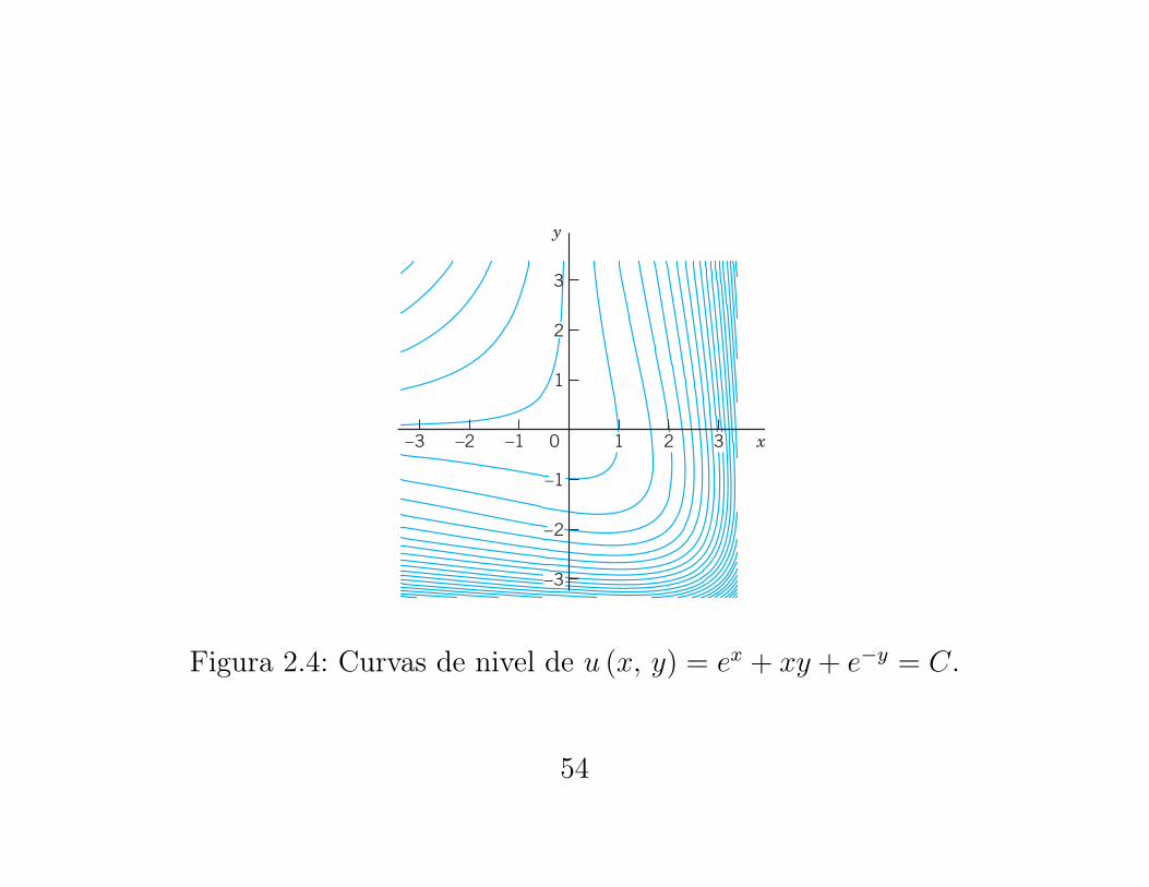
Paso3 Solución particular: La condición inicial y (0) = �1 implica queu (0, �1) = 1 + e = 3.72. Por lo tanto la solución al problema devalor inicial es
u (x, y) = e
x
+ xy + e
�y
= 1 + e = 3.72 .
(ver Figura 2.4).
2.5. EDOs linealesUna EDO de primer orden es lineal si se puede escribir de la forma
y
0+ p (x) y = r (x) . (2.11)
Esta ecuación es lineal en y y en y
0. Las funciones p (x) y r (x) puedenser funciones arbitrarias de x.
53
Test for exactness; you will get 1 on both sides of the exactness condition. By integration, using (4a),
Differentiate this with respect to y and use (4b) to get
Hence the general solution is
Setp 3. Particular solution. The initial condition gives Hence theanswer is Figure 18 shows several particular solutions obtained as level curvesof obtained by a CAS, a convenient way in cases in which it is impossible or difficult to cast asolution into explicit form. Note the curve that (nearly) satisfies the initial condition.
Step 4. Checking. Check by substitution that the answer satisfies the given equation as well as the initialcondition. !
u(x, y) ! c,ex " xy " e!y ! 1 " e ! 3.72.
u(0, #1) ! 1 " 0 " e ! 3.72.y(0) ! #1
u(x, y) ! ex " xy " e!y ! c.
k ! e!y " c*.dkdy
! #e!y,0u0y
! x "dkdy
! N ! x # e!y,
u ! !(ex " y) dx ! ex " xy " k(y).
26 CHAP. 1 First-Order ODEs
y
x0–1–2–3
1
3
1 2 3
–1
–2
–3
2
Fig. 18. Particular solutions in Example 5
1–14 ODEs. INTEGRATING FACTORS Test for exactness. If exact, solve. If not, use an integratingfactor as given or obtained by inspection or by the theoremsin the text. Also, if an initial condition is given, find thecorresponding particular solution.1.2.3.4.5.6.7. 2x tan y dx " sec2 y dy ! 0
3(y " 1) dx ! 2x dy, (y " 1)x!4
(x2 " y2) dx # 2xy dy ! 0e3u(dr " 3r du) ! 0sin x cos y dx " cos x sin y dy ! 0x3dx " y3dy ! 02xy dx " x2 dy ! 0
8.
9.
10.
11. 2 cosh x cos y
12.
13.
14.
15. Exactness. Under what conditions for the constants a,b, k, l is exact? Solvethe exact ODE.
(ax " by) dx " (kx " ly) dy ! 0
F ! xayb(a " 1)y dx " (b " 1)x dy ! 0, y(1) ! 1,
e!y dx " e!x(#e!y " 1) dy ! 0, F ! ex"y
(2xy dx " dy)ex2
! 0, y(0) ! 2
dx ! sinh x sin y dy
y dx " 3y " tan (x " y)4 dy ! 0, cos (x " y)
e2x(2 cos y dx # sin y dy) ! 0, y(0) ! 0
ex(cos y dx # sin y dy) ! 0
P R O B L E M S E T 1 . 4
c01.qxd 7/30/10 8:15 PM Page 26
Figura 2.4: Curvas de nivel de u (x, y) = e
x
+ xy + e
�y
= C.
54

2.5.1. EDO lineal homogénea
Cuando en el intervalo J = {x 2 R | a < x < b} el término r (x) ⌘ 0
en J la EDO (2.11) se convierte en
y
0+ p (x) y = 0 ,
y se denomina homogénea. Separando variables e integrando se obtiene
dy
y
= �p (x) dx ) ln |y| = �ˆ
p (x) dx+ C
⇤.
Tomando exponentes en ambos lados obtenemos la solución general dela ecuación homogénea
y (x) = Ce
�´p(x)dx
.
Si se elige C = 0 se obtiene la solución trivial y (x) = 0 en el intervaloJ .
55

2.5.2. EDO lineal no homogénea
Ahora resolvemos la EDO (2.11) en el caso en que r (x) no es ceroen el intervalo J , en cuyo caso (2.11) es no homogénea.
Método de solución: (2.11) tiene un Factor de Integración F = F (x)
(que depende solo de x). Se puede hallar mediante el Teorema 2.12 odirectamente.
Procedemos Directamente:
Se multiplica (2.11) por F (x)
Fy
0+ Fpy = Fr . (2.12)
El lado izquierdo es la derivada (Fy)
0= F
0y + Fy
0 del productoFy si
pFy = F
0y ) pF = F
0.
56
Por separación de variables
dF
F
= pdx ) ln |F | = h ,ˆ
pdx ) F = e
h
.
Dada esta F y con h
0= p la EDO (2.12) se convierte en
e
h
y
0+ e
h
py = e
h
y
0+
�e
h
�0y =
�e
h
y
�0= e
h
r .
Por integración
e
h
y =
ˆe
h
r + C .
Dividiendo por e
hse obtiene la expresión deseada
y (x) = e
�h
C + e
�h
´e
h
r , h =
ˆp (x) dx . (2.13)
Esto reduce la tarea de resolver la EDO (2.11) a la de evaluarintegrales.
57

Nótese que en (2.13):
1. La constante de integración de h no afecta el resultado.
2. Dada una Condición Inicial (C.I.), la única cantidad que dependede esta C.I. es C.
3. La respuesta total es la suma de dos términos: La respuesta a laC.I. + La respuesta a la entrada r (x)
y (x) = e
�h
C| {z }Rpta a C.I.
+ e
�h
ˆe
h
r
| {z }Rpta a entrada r
Ejemplo 2.15 Resuelva el Problema de Valores Iniciales
y
0+ y tan x = sin 2x , y (0) = 1 .
58
Solución: Aqui p = tan x, r = sin 2x = 2 sin x cos x, y
h =
ˆpdx =
ˆtan xdx = ln |sec x| .
De aqui vemos que en (2.13)
e
h
= secx , e
�h
= cosx , e
h
r = (secx) (2 sin x cos x) = 2 sin x ,
y la solución general de la EDO es
y (x) = cos x
✓2
ˆsin x dx+ C
◆= C cos x� 2 cos
2x .
De la C.I.
y (0) = 1 ) 1 = C cos 0� 2 cos
20 = C � 2 ) C = 3 ,
y la solución del Problema de Condiciones Iniciales es
y (x) = 3 cosx| {z }Rpta a C.I.
�2 cos
2x| {z }
Rpta a entrada sin 2x
.
59
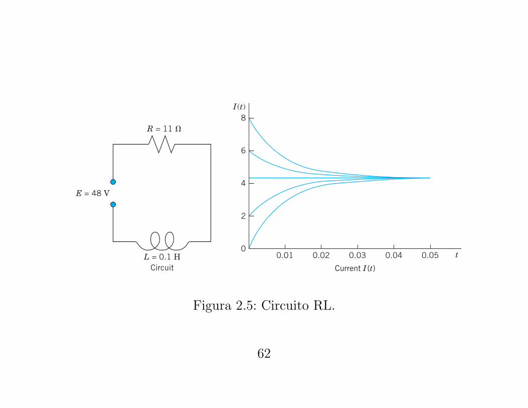
Ejemplo 2.16 Circuito EléctricoModele el circuito RL de la Figura 2.5 y resuelva la EDO resultante
para la corriente I (t) (en Amperios A), dónde t es el tiempo. Asuma queel circuito tiene como Fuente de Voltaje E (t) a una batería de E = 48
V (Voltios) constante, una resistencia de R = 11 ⌦ (ohmios) y unainductancia de L = 0.1 H (Henrios) y que la corriente inicial es cero.
Solución: De acuerdo a las leyes de Kirchhoff se tiene que
LI
0+RI = E (t) ) I
0+
R
L
I =
E (t)
L
.
Se puede obtener la solución general de esta EDO de (2.13) con x = t,y = I, p =
R
/L, h = (
R
/L) t
I (t) = e
�RL t
✓C +
ˆe
RL t
E (t)
L
dt
◆.
60

Integrando
I (t) = e
�RL t
✓C +
E
L
L
R
e
RL t
◆= e
�RL t
C +
E
R
= e
�110tC +
48
11
.
La C.I. I (0) = 0 implica
I (0) = e
0
✓C +
E
R
e
0
◆= 0 ) C = �E
R
,
así que la solución particular es
I (t) = �e
�110t48
11
+
48
11
=
48
11
�1� e
�110t�.
61
30 CHAP. 1 First-Order ODEs
We can solve this linear ODE by (4) with obtaining the general solution
By integration,
(7)
In our case, and thus,
In modeling, one often gets better insight into the nature of a solution (and smaller roundoff errors) by insertinggiven numeric data only near the end. Here, the general solution (7) shows that the current approaches the limit
faster the larger is, in our case, and the approach is very fast, frombelow if or from above if If the solution is constant (48/11 A). SeeFig. 19.
The initial value gives and the particular solution
(8)!
I !ER
(1 " e!(R>L)t), thus I !4811
(1 " e!110t).
c ! "E>RI(0) ! E>R # c ! 0,I(0) ! 0
I(0) ! 48>11,I(0) $ 48>11.I(0) % 48>11R>L ! 11>0.1 ! 110,R>LE>R ! 48>11
I ! 4811 # ce!110t.
E(t) ! 48>0.1 ! 480 ! const;R>L ! 11>0.1 ! 110
I ! e!(R>L)t aEL
e1R>L2t
R>L # cb !ER
# ce!(R>L)t.
I ! e!(R>L)t a !e(R>L)t
E(t)L
dt # c b.x ! t, y ! I, p ! R>L, h ! (R>L)t,
Fig. 19. RL-circuit
E X A M P L E 3 Hormone Level
Assume that the level of a certain hormone in the blood of a patient varies with time. Suppose that the time rateof change is the difference between a sinusoidal input of a 24-hour period from the thyroid gland and a continuousremoval rate proportional to the level present. Set up a model for the hormone level in the blood and find itsgeneral solution. Find the particular solution satisfying a suitable initial condition.
Solution. Step 1. Setting up a model. Let be the hormone level at time t. Then the removal rate is The input rate is where and A is the average input rate; here to makethe input rate nonnegative. The constants A, B, K can be determined from measurements. Hence the model is thelinear ODE
The initial condition for a particular solution is with suitably chosen, for example, 6:00 A.M.
Step 2. General solution. In (4) we have and Hence (4) gives thegeneral solution (evaluate by integration by parts)"eKt cos vt dt
r ! A # B cos vt.p ! K ! const, h ! Kt,
t ! 0ypart(0) ! y0ypart
yr(t) ! In " Out ! A # B cos vt " Ky(t), thus yr # Ky ! A # B cos vt.
A & Bv ! 2p>24 ! p>12A # B cos vt,Ky(t).y(t)
L = 0.1 HCircuit Current I (t)
I (t)
E = 48 V
R = 11 '
0.01 0.02 0.03 0.04 0.05 t
2
4
6
8
0
c01.qxd 7/30/10 8:15 PM Page 30
Figura 2.5: Circuito RL.
62

2.6. ODE de Bernoulli: Reducción a una ODELineal
La Ecuación de Bernoulli es
y
0+ p (x) y = g (x) y
a
, a 2 R . (2.14)
Si a = 0 o a = 1 la ODE (2.14) es lineal. En todos los demás casos esno lineal.
Usando la transformación
u (x) = [y (x)]
1�a
,
se obtiene que
u
0= (1� a) y
�a
y
0= (1� a) y
�a
(gy
a � py) = (1� a)
�g � py
1�a
�)
) u
0+ (1� a) pu = (1� a) g ,
que es una EDO Lineal.63

Ejemplo 2.17 Ecuación LogísticaResuelva la siguiente ecuación de Bernoulli, conocida como Ecua-
ción Logística (o Ecuación de Verhulst):
y
0= Ay � By
2.
Solución: En este caso a = 2 y el cambio de variable es u = y
1�a
=
y
�1. Para uobtenemos
u
0= �y
�2y
0= �y
�2�Ay � By
2�= B � Ay
�1 )
) u
0+ Au = B .
La solución general es
u = Ce
�At
+
B
A
) y (t) =
1
u (t)
=
1
Ce
�At
+
B
A
.
64

SEC. 1.5 Linear ODEs. Bernoulli Equation. Population Dynamics 33
Fig. 21. Logistic population model. Curves (9) in Example 4 with A>B ! 4
1 2 3 4
Population y
Time t
2
0
= 4
6
8
AB
Population DynamicsThe logistic equation (11) plays an important role in population dynamics, a fieldthat models the evolution of populations of plants, animals, or humans over time t.If then (11) is In this case its solution (12) is and gives exponential growth, as for a small population in a large country (theUnited States in early times!). This is called Malthus’s law. (See also Example 3 inSec. 1.1.)
The term in (11) is a “braking term” that prevents the population from growingwithout bound. Indeed, if we write we see that if then
so that an initially small population keeps growing as long as But ifthen and the population is decreasing as long as The limit
is the same in both cases, namely, See Fig. 21.We see that in the logistic equation (11) the independent variable t does not occur
explicitly. An ODE in which t does not occur explicitly is of the form
(13)
and is called an autonomous ODE. Thus the logistic equation (11) is autonomous.Equation (13) has constant solutions, called equilibrium solutions or equilibrium
points. These are determined by the zeros of because gives by(13); hence These zeros are known as critical points of (13). Anequilibrium solution is called stable if solutions close to it for some t remain closeto it for all further t. It is called unstable if solutions initially close to it do not remainclose to it as t increases. For instance, in Fig. 21 is an unstable equilibriumsolution, and is a stable one. Note that (11) has the critical points and
E X A M P L E 5 Stable and Unstable Equilibrium Solutions. “Phase Line Plot”
The ODE has the stable equilibrium solution and the unstable as the directionfield in Fig. 22 suggests. The values and are the zeros of the parabola in the figure.Now, since the ODE is autonomous, we can “condense” the direction field to a “phase line plot” giving and
and the direction (upward or downward) of the arrows in the field, and thus giving information about thestability or instability of the equilibrium solutions. !y2,
y1
f (y) ! (y " 1)(y " 2)y2y1
y2 ! 2,y1 ! 1yr ! (y " 1)(y " 2)
y ! A>B.y ! 0y ! 4
y ! 0
y ! const.yr ! 0f (y) ! 0f (y),
yr ! f (y)
yr ! f (t, y)
A>B.y # A>B.yr $ 0y # A>B,
y $ A>B.yr # 0,y $ A>B,yr ! Ay 31 " (B>A)y4,"By
2
y ! (1>c)eAtyr ! dy>dt ! Ay.B ! 0,
c01.qxd 7/30/10 8:15 PM Page 33
Figura 2.6: Modelo de población Logístico. Curvas con A
/B = 4.
Podemos ver que y ⌘ 0 (y (t) = 0 para todo t) es también unasolución.
65

Bibliografía
[1] Erwin Kreyszig. Advanced Engineering Mathematics. 10th Edition.New York: Academic Press, 1975.
[2] Wolfgang Walter. Gewöhnliche Differentialgleichungen: Eine Ein-führung. 7. Auflage, Springer-Verlag, 2000.
[3] https://en.wikipedia.org/wiki/Equation
66
[4] https://en.wikipedia.org/wiki/Operation_(mathematics)
67
Top Related