Entropic landscape

Entropic landscape

Raphael Bousso1,2,3 and Roni Harnik4

1Center for Theoretical Physics, Department of Physics, University of California, Berkeley, California 94720-7300, USA2Lawrence Berkeley National Laboratory, Berkeley, California 94720-8162, USA3Institute for the Physics and Mathematics of the Universe, University of Tokyo,

5-1-5 Kashiwa-no-Ha, Kashiwa City, Chiba 277-8568, Japan4Stanford Institute for Theoretical Physics, Department of Physics, Stanford University, California 94305, USA

(Received 12 August 2010; published 21 December 2010)

We initiate a quantitative exploration of the entire landscape. Predictions thus far have focused on

subsets of landscape vacua that share most properties with our own. Using the entropic principle (the

assumption that entropy production traces the formation of complex structures such as observers), we

derive six predictions that apply to the whole landscape. Typical observers find themselves in a flat

Universe, at the onset of vacuum domination, surrounded by a recently produced bath of relativistic

quanta. These quanta are neither very dilute nor condensed, and thus appear as a roughly thermal

background. Their characteristic wavelength is of order the inverse fourth root of the vacuum energy.

These predictions hold for completely arbitrary observers, in arbitrary vacua with potentially exotic

particle physics and cosmology. They agree with observation: We live in a flat Universe at the onset of

vacuum domination, whose dominant entropy production process (the glow of galactic dust) has recently

produced a radiation bath (the cosmic infrared background). This radiation is marginally dilute,

relativistic, and has a wavelength of order 100 microns, as predicted.

DOI: 10.1103/PhysRevD.82.123523 PACS numbers: 98.80.Cq

I. INTRODUCTION

A. Predictions in the multiverse

In a theory that gives rise to an eternally inflating multi-verse, such as string theory [1,2], we must compute notwhat is typical, but what is typically observed. Cosmichorizons prevent observers from seeing all but a finiteportion of the multiverse, near the vantage point at whichthey happen to find themselves. The likely properties oftheir local environment depend not only on the relativeabundance of different properties in the landscape ofvacua, but also on correlations between these properties(such as the amount of vacuum energy) and the localabundance of observers.

It is impractical to compute the number of observers indifferent regions from first principles. However, one mayargue that the number of observers of a certain class isproportional to the abundance of some object necessaryfor their existence, such as galaxies, stars, carbon nuclei,complex organic molecules, etc. (This class of observershad better include us, for otherwise our observations wouldnot test the computed predictions.) However, this reasoningexcludes from consideration observers that are outside thespecific class, ones that are qualitatively very differentfrom us, and do not require the object that was deemednecessary. By extension, this will exclude vacua in whichonly such ‘‘exotic’’ observers exist. Nevertheless, thisapproach is perfectly sensible. By computing what it typi-cally observed by observers that are, in some way, like us,we may well falsify a given multiverse theory. If ourobservations turn out to be atypical even within a restrictedclass of observers and vacua (for example, if we found that

the observed value of the cosmological constant is manystandard deviations from the mean value found by observ-ers that live on galaxies), then the theory will be disfavoredat the corresponding level of confidence.Conditioning on observers ‘‘like us’’ does impose limi-

tations. What we condition on, we cannot predict. Whenwe restrict attention to a special class of observers and toa small fraction of the landscape, we cannot explain whywe find ourselves in this particular class. And once amultiverse theory has been supported by showing that ourobservations are typical in some restricted class, one wouldlike to test the theory further by asking whether they aretypical in a wider class of observers. The fewer conditionswe impose, the more is left to predict, and the moreopportunities we will have to falsify the theory.Using the causal diamond1 measure [3] for regulating

the divergences of eternal inflation, a prediction that tran-scends this limitation was recently derived [4]: Observersthat live at a time tobs after the formation of their vacuumbubble are likely to measure a cosmological constant oforder

�� t�2obs: (1.1)

With tobs � 1010 yr� 1061, the time at which we happen tolive, the predicted value of� agrees well with the observedvalue,

1The causal diamond is the intersection of the causal past of amaximally extended timelike geodesic (in a long-lived de Sittervacuum, this is simply the interior of the event horizon) with thefuture of a point on the reheating surface. The causal diamondmeasure is reviewed in the Appendix.

PHYSICAL REVIEW D 82, 123523 (2010)

1550-7998=2010=82(12)=123523(19) 123523-1 � 2010 The American Physical Society

http://dx.doi.org/10.1103/PhysRevD.82.123523

�o ¼ 3:7� 10�122: (1.2)

(Unless explicit units are displayed, Planck units are usedin this paper.)

Though this point was not emphasized in Ref. [4], wenote here that the relation (1.1) is (statistically) predictedfor all observers, whether or not they are in any sense ‘‘likeus,’’ and whether or not they live in vacua where words like‘‘Galaxy’’ or ‘‘carbon’’ even make sense. In particular,Eq. (1.1) is predicted to hold independently of the actualvalue of tobs. Thus, the result solves the coincidence (‘‘whynow’’) problem completely generally, predicting that typi-cal observers find themselves at the onset of vacuumdomination. These claims may seem strong, so let us verifythem by reviewing the basic argument leading to Eq. (1.1),and demonstrating that it is independent of the nature ofobservers.

In vacua with small cosmological constant (� � t�2obs),

vacuum energy is dynamically irrelevant at and before thetime tobs and so, in particular, cannot affect the number ofobservers. In this range of �, the probability distribution isgoverned by the prior landscape distribution, which growstowards larger values of �, like �. In vacua with largecosmological constant (� � t�2

obs), the number of observ-

ers in the causal diamond is at least exponentially sup-pressed due to the depletion of the total mass by the

de Sitter expansion, like expð� ffiffiffiffiffiffiffi3�

ptobsÞ [4]. In this range,

the probability distribution favors smaller values of �, sothe overall distribution peaks near �� t�2

obs. Now, it is

possible that sufficiently large values of the cosmologicalconstant disrupt the formation of observers altogether (e.g.,for observers like us, by disrupting galaxy formation).Whether this happens, and for what values of �, willindeed depend on the type of observers and the dynamicalprocesses that lead to their formation. But any such addi-tional suppression can only occur if� has some dynamicaleffect before tobs, i.e., for values of � greater than t�2

obs.

Since the distribution is already suppressed in this regime,this will not significantly affect the prediction, Eq. (1.1).

Let us summarize the two reasons why Eq. (1.1) is a verygeneral prediction: (1) both � and tobs are well-definedobservable quantities in any semiclassical vacuum—unlike, for example, the number of galaxies or carbonatoms; and (2) no additional vacuum-specific assumptionswent into deriving their correlation, Eq. (1.1); in particular,no assumption about the nature of the observers was made,and no necessary condition for their existence was posited.Unfortunately, examination of the argument in the previousparagraph suggests that this fortuitous circumstance isquite peculiar to the pair of variables appearing inEq. (1.1). Perhaps a few other examples can be found.But short of demonstrating that a certain property cannotoccur at all in the entire vacuum landscape [5], it does notseem likely that many predictions can be made withoutassuming anything about observers.

This does not mean that we must give up on exploringthe whole landscape. Rather, the challenge is to identify auniversal necessary condition for observers: one that isplausible but not so specific as to restrict the class ofobservers, or the class of vacua, that can be considered.Galaxies or carbon may be good proxies for observers inrestricted classes of vacua, with their abundance trackingthe true number of observers reasonably well. But they willnot do for this more ambitious purpose.

B. The entropic principle

In Ref. [3], a novel proxy for observers was proposed:the production of matter entropy. The formation of anycomplex structure (and thus, of observers, in particular), isnecessarily accompanied by an increase in the entropy ofthe environment. Thus, entropy production is a necessarycondition for the existence of observers. In a regionwhere no entropy is produced, no observers can form.The ‘‘entropic principle’’ is the assumption that the numberof observers is proportional, on average, to the amount ofentropy produced:

nobs / �S: (1.3)

Entropy production is obviously not sufficient for theexistence of observers, just as galaxies are not sufficient.The entropic principle makes no claim of establishing anequivalence where previously only a necessary conditionwas known. Rather, its potential advantage lies in theuniversality of the notion of entropy. A galaxy, or anorganic molecule, is an imprecise and highly derivativeconcept with no obvious analogue in vacua with differentcosmology, particles or forces. Matter entropy, by contrast,is defined in any vacuum that admits a semiclassical de-scription.2 Therefore, its use as a proxy does not require usto restrict our attention to a small subset of the landscape.Before applying the entropic principle on the whole

landscape (the purpose of the present paper), let us checkwhether entropy production makes for a good proxy invacua like ours, where we have alternative, more conven-tional methods of estimating the abundance and spacetimedistribution of observers. Beginning with our own vacuum,let us pretend, for a moment, that we do not alreadyknow our position in space and time, and use the entropic

2In particular, matter entropy can be distinguished from theBekenstein-Hawking entropy associated with black hole orcosmological horizons, in the semiclassical regime. We do notinclude horizon entropy in �S. This is legitimate, since we arenot claiming that entropy production is fundamentally equivalentto observation; we are merely interested in exploring matterentropy production as a proxy for observers that can be definedin all vacua. However, it is worth noting that the distinctionbetween matter and horizon entropy is particularly natural in thecontext of the causal patch and causal diamond measures. Thecosmological horizon and the horizons of all black holes are bydefinition on or just outside the boundary of the causal patch, andso are automatically excluded from consideration.

RAPHAEL BOUSSO AND RONI HARNIK PHYSICAL REVIEW D 82, 123523 (2010)

123523-2

principle to ‘‘predict’’ our location. Analysis of a variety ofknown astrophysical processes [4] shows that the entropyproduction in the causal diamond in our Universe is domi-nated by the infrared photons emitted by dust heated bystarlight. According to the entropic principle, this impliesthat typical observers should find themselves near stars ingalaxies (and not, for example, in a more generic locationlike intergalactic space). The rate of entropy productionpeaks at a time of order 1010 years [4], so the entropicprinciple predicts that we should find ourselves living atabout that time. Both of these predictions are correct,which suggests that the entropy production is indeed auseful proxy for observers.

Next, consider an ensemble of vacua that includes ourown, as well as (a) vacua like ours except without complexmolecules, (b) vacua like ours but without stars, and(c) vacua like ours but without galaxies. In our vacuum,dust scatters a fraction of order 1 of stellar photons,converting each optical photon into about 100 infraredphotons. Vacua of type (a) do not contain dust, which iscomposed of large organic molecules [6,7]. Therefore, theentropy production in vacua without organic chemistry isabout 100 times smaller than in our vacuum. In vacuawithout stars, the entropy is even smaller (dominated,perhaps, by active galactic nuclei, if those still exist, orby galaxy cooling); and without galaxies, �S is smallerstill. This shows that�S is remarkably sensitive to some ofthe rather specific criteria that have been conjectured to benecessary for life of our type. This further boosts ourconfidence that it will be a useful proxy in the largerlandscape.

C. Outline

In this paper, we will study the implications of theentropic principle applied to the landscape as a whole.The basic idea is simple: if entropy production tracesobservers, then most observers should find themselvesin an environment in which a lot of entropy is produced.The question is how to turn this insight it into quantitativepredictions of observable quantities. Our approach will beto define a set of observables xi that characterize processesthat produce entropy, and to study how �S depends on theparameters xi. By the entropic principle, one expects thatmost observers will be witness to a process that comesclose to maximizing the amount of entropy production.Thus, we predict that the observed values of the parametersxi are not far from the values that maximize �S.

In Sec. II, we define six scanning parameters: the time ofentropy production, tburn; the characteristic wavelength ofthe quanta carrying the entropy, �; the volume fractionoccupied by the quanta, fV , which is small if quanta aredilute; the characteristic occupation number, �, whichquantifies the typical overlap between entropic quanta;the spatial curvature, parametrized by the time of curvaturedomination, tc, and the rest mass of entropic quanta, m.

In order to be able to judge the sharpness of the predictionswe will later derive from the causal entropic principle, wediscuss the considerable range of values that can be takenin principle by each parameter.In Sec. III, we consider a (nearly) arbitrary entropy

production process: free energy is converted into (nearly)arbitrary quanta, which we refer to as ‘‘entropic quanta.’’We consider a vacuum with cosmological constant �,which we treat as an input parameter much like tobs inthe example of Eq. (1.1). By maximizing the entropyproduced, �S, over our scanning parameters, we obtainpredictions for all six parameters.In Sec. IV, we consider concrete examples processes that

produce entropy. This demonstrates explicitly that entropyproduction is smaller than the maximal value in universesthat burn up too little of their rest mass, or produce onlyclassical radiation, or produce thermal radiation at a tem-perature that is higher or lower than optimal.In Sec. V, we turn to our own Universe and compare our

predictions to the values that we observe for the scanningparameters tburn, �, fV , �, tc, m. (We briefly summarizeour predictions, and how they compare to observation, inSec. I D immediately below.)We finish in Sec. VI by discussing our results and

considering future extensions. We sketch a statistical ex-planation of the near-coincidence between the temperatureof the cosmic microwave background and the cosmicinfrared background, for which no natural explanation isknown. We also consider what happens if � is allowed toscan: we argue that the observed value of the cosmologicalconstant may be directly related to the number of vacua inthe landscape, providing a fundamental hierarchy to whichother known hierarchies are correlated.The Appendix contains a brief review of the definition of

the causal diamond measure.

D. Summary of results

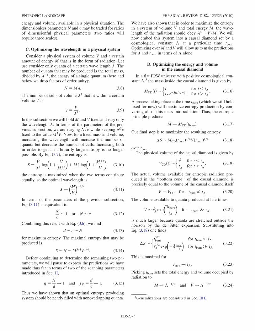
Let us briefly summarize our predictions and how theycompare to observation (see Fig. 1):

(1) Prediction: tburn � t� � j3=�j1=2: Most of the en-tropy in the causal diamond is produced aroundthe onset of vacuum domination at the time t�. Bythe entropic principle, this is equivalent to the pre-diction that observers should find themselves at theonset of vacuum domination, and thus, to Eq. (1.1).Observation: The dominant entropy production pro-cesses that we observe or infer from observationtake place around 3:5 Gyr� 1060:3 after the bigbang [4]. (Of these, the most important is theemission of infrared radiation by galactic dust.)In our Universe, t� � 1060:3, so the prediction isaccurate.

(2) Prediction: �� j�j�1=4: The characteristic energyof the quanta of matter carrying this entropy is oforder the energy scale of the vacuum.

ENTROPIC LANDSCAPE PHYSICAL REVIEW D 82, 123523 (2010)

123523-3

Observation: The energy of quanta emitted bygalactic dust is observed to be about 300 �m�1031:3, which is indeed of order ��1=4 � 1030:8.

(3) Prediction: �� 1: The quanta produced by thisprocess are dilute, in the sense that occupationnumbers are of order unity. The quanta are not inclassical radiation, which would have � � 1.Observation: Experimentally, we know that dustwill not give off classical radiation when scatteringoptical photons, so �� 1.

(4) Prediction: fV � 1: Entropic quanta are nearlydense in space. Therefore, they will be observed asa steady flux of radiation, rather than as bursts,and they will appear to come from a large fractionof the sky.Observation: We observe the glow of galactic dustfrom the Universe as a roughly isotropic cosmicinfrared background (CIB) which is steady to withinthe time resolution of current detectors. Given theflux and wavelength of the CIB we can howeverdeduce that it is somewhat dilute, with an fV �0:5� 10�4. Given that fV may a priori span over180 orders of magnitude, this value is remarkablyclose to 1.

(5) Prediction: The universe is not curvature domi-nated, i.e., the radius of spatial curvature is larger

than the Hubble radius.

Observation: Curvature does not dominate. The

curvature radius is at least 10 times larger than the

Hubble radius [8].(6) Prediction: The quanta produced by this process are

relativistic.Observation: The cosmic infrared background

consists of photons, i.e., of massless particles, which

are obviously relativistic.Let us give a rough explanation of how the entropic

principle, combined with the causal diamond cutoff, leadsto the above predictions. The causal diamond contains themost mass (which is an upper bound on free energy) at thetime t�, so this is the best era in which to produce entropyby burning up free energy. For a dilute gas of quanta, theentropy is proportional to the number of quanta produced,which is given by the free energy divided by the energy perquantum: S� N �M�. To maximize the entropy, there-fore, one would like to make the wavelength � large. Butthis also increases the volume occupied by each quantum.The total volume the quanta can occupy is limited bycausality, so for � sufficiently large the quanta can no

energyconservation

single quantum

S

1 1010 1020 1030 1040 1050 106010 183

10 152

10 121

90

59

28

f V

S

energy conservation

1 1011 1022 1033 1044 10550.01

1019

1040

1061

1082

10103

tburn

FIG. 1 (color online). Two slices of our parameter space: the ð�; fVÞ plane on the left, and the ðtburn; �Þ plane on the right. In eachplot, the remaining parameters are held fixed at their optimal values. The axes show the possible values these parameters may take (inPlanck units), in vacua with our value of the cosmological constant. The shaded regions are unphysical, either because the energy ofthe entropic radiation exceeds the total mass within the causal diamond, or because there is less than one quantum of radiation inthe diamond. The dashed contours are surfaces of constant entropy (10 orders of magnitude apart in entropy) and the black arrowrepresents the direction in which entropy production increases. The optimal values, for which entropy production is maximized,are shown as a black dot. The observed values in our Universe are shown as a red open circle; as predicted by the entropic principle,they are very close to the optimal values. (The black dot cannot be seen in the figure on the right because it is covered by the redcircle.)


123523-4

longer be dilute, but would have to overlap (� � 1). This

happens when ��1=4. Increasing the number of quantabeyond this point is unfavorable to entropy production.(This is most obvious in the extreme limit where�� N and S ¼ logN.) Thus, the entropy is maximizedwhen the photons make use of all available volume, fV � 1while remaining marginally dilute, �� 1. Curvature isdisfavored because it decreases the maximum volumeavailable to the entropic radiation. Nonrelativistic quantaare disfavored because some of the mass inside the causaldiamond goes into the rest mass of particles, decreasing thenumber of quanta that can be produced.

II. PARAMETERS AND THEIR RANGES

Consider a Friedmann-Robertson-Walker (FRW) uni-verse with cosmological constant �, which is taken to bea fixed input parameter. We will now define six scanningparameters (tburn, �, fV , �, tc, m), which can be used tocharacterize entropy production in arbitrary vacua, andwhose values we will later predict in terms of �.

Entropy is produced by an arbitrary process, during anera tburn, in the form of quanta of rest mass m, withcharacteristic wavelength � per quantum. We will referto the carriers of this entropy as entropic quanta or collec-tively as entropic radiation. In the following discussion, wewill neglect factors of order unity. We define fV to bethe fraction of volume occupied by entropic radiation.We define � as the characteristic occupation number ofentropic quanta, in the regions occupied by at least onesuch quantum. (One could also consider an occupationnumber averaged over all space, which would be fV� inour notation. However, it will be more convenient to workwith the above definition.) Finally, we define tc as the timewhen (open or closed) spatial curvature would begin todominate the evolution of the universe if the cosmologicalconstant were zero. That is tc is the actual time of curvature

domination if tc < t� ��1=2; for tc > t�, curvaturenever dominates after reheating, and the universe can beconsidered spatially flat on the scale of the causal diamond.

Let us examine the range of values each scanningparameter can take. The time tburn cannot be smaller thanthe Planck time. One might think that it can take arbitrarily

large values. However, after a time t� � ð�=3Þ�1=2, theuniverse begins to accelerate its expansion. As matter exitsfrom the de Sitter horizon, the total mass of matter in thecausal diamond drops like t� expð�3t=t�Þ. This becomesless than the smallest reasonable quantity of mass thatcan be defined, a quantum of wavelength t�, whenexpð3t=t�Þ � t2�. Thus, we find that

1 � tburn � 23t� logt�: (2.1)

For example, in vacua with our value of the cosmologicalconstant, � ¼ �o ¼ 3:72� 10�122, this implies that tburncan range over 63 orders of magnitude. (In Sec. III E 3 we

will address nonhomogeneities that can in principle maketburn even larger.)The wavelength of entropic quanta cannot be smaller

than the Planck length or larger than the de Sitter horizon:

1 � � � t�; (2.2)

with � ¼ �o, this implies that � can range over 61 ordersof magnitude.The volume fraction occupied by radiation, fV , cannot

exceed 1 (by definition). The smallest it can be is 1=V,where V is the total volume available; this corresponds toa single quantum of Planck size. The maximum volumeof the causal diamond in a universe with cosmologicalconstant � is of order t3�, so

t�3� � fV � 1: (2.3)

This corresponds to a range of 183 orders of magnitude invacua with � ¼ �o.The typical occupation number in regions containing

entropic radiation, �, cannot be less than 1 by definition;and it cannot be larger than the total number of quanta, N.As we will discuss in more detail in Sec. III, the total massinside the causal diamond is maximal around the time t�,when it is given by t�. The smallest possible mass of asingle quantum is t�1

� (which is attained when its wave-

length is as large as the universe). The largest possible Ncorresponds to dividing the maximum total mass in theuniverse by the energy of the smallest possible quanta.This yields N � t2� and corresponds to a condensate of

� ¼ N quanta, each of horizon size, sitting on top of oneanother. Thus,

1 � � � t2�; (2.4)

corresponding to a range of 122 orders of magnitude invacua with � ¼ �o.The rest mass of the species carrying the entropic radia-

tion can range from the Planck mass down to zero mass,and so has infinite range in principle. In practice, it isunclear how one would measure the mass of a particlewhose Compton wavelength exceeds the largest causallyaccessible scale, t�, so we take the mass range to be

m ¼ 0 or t�1� � m � 1: (2.5)

This corresponds to 61 orders of magnitude in vacua with� ¼ �o (plus the special case of massless particles, whichwe shall see is actually the main carrier of entropic radia-tion in our universe).The curvature time scale, tc, ranges in practice from the

time of reheating (which could be as early as the Plancktime) to the time of vacuum domination, t�; larger valuesof tc correspond to a universe which always appears flat onthe horizon scale. Thus,

1 � tc � t�; (2.6)


123523-5

corresponding to a range of 61 orders of magnitude invacua with � ¼ �o.

We summarize our parameters and their range in thefollowing Table I: Thus we are considering a six-dimensional parameter space, with each parameter allowedan enormous range a priori. This should be kept in mindin order to appreciate the accuracy of the predictions ofthe entropic principle, which we derive next. Note thateach point in the parameter space can correspond to ahuge variety of different entropy production processes.We have not specified how the entropic radiation is actuallygenerated, so that our analysis remains sufficiently generalto apply to all semiclassical landscape vacua.

III. ENTROPYAND ITS MAXIMIZATION

A. The entropy of quanta in a grid

The standard method of doing statistical mechanics of anoninteracting gas of particles is to compute the expectedoccupation numbers of the one-particle energy eigenstates,or ‘‘orbitals,’’ in a box. These numbers are interpreted asthe number of photons (or quanta of some other field) ofthe corresponding energy. These states, however, havesupport over the entire volume of the box and are(by definition) exactly time-independent. One of the keyobservables studied in this paper is the volume fractionoccupied by the radiation, so this basis is not well-suited toour purposes. Therefore, we will use a basis of one-particlestates which are not energy eigenstates but are localizedin space. At a given characteristic wavelength (whosevariation we will consider later) we may consider a gridconsisting of c cells of size �3. The volume fraction definedin the previous section can be represented as

fV � d

c; (3.1)

where d is the number of cells containing at least onequantum (‘‘occupied’’ cells). The characteristic occupationnumber is

� � N

d: (3.2)

Given N, c, and d (or equivalently, N, fV and �), theentropy is

S ¼ logðN fN �Þ; (3.3)

where

N f ¼ cd

� �(3.4)

is the number of different ways of choosing the d occupiedcells from among the c cells, and

N � ¼ N � 1d� 1

� �(3.5)

is the number of different ways of distributing N � dquanta among the d occupied cells. (By definition, eachoccupied cell contains at least one quantum, so only theremaining N � d quanta are left to be distributed freely.)We will be assuming that N, c, and d are all much greaterthan one, so that the�1 terms can be neglected in Eq. (3.5).

B. Optimizing the distribution of quanta

While holding fixed the number of quanta, N, and thenumber of cells, c, let us ask for what value of d the entropyis maximized. This occurs when Sðdþ 1Þ ¼ SðdÞ, or, fromEqs. (3.4) and (3.5), when

d ¼ Nc

N þ c; (3.6)

where we have neglected terms of order unity both in thenumerator and denominator. As one would intuitivelyguess, entropy is maximized when the number of occupiedcells d is as large as possible, set either by the number ofcells c or by the number of quanta N, whichever is smaller.After picking the optimal value for d from Eq. (3.6) theentropy is

S ¼ c log

�N þ c

N

�þ N log

�N þ c

c

�; (3.7)

where we have employed the Stirling formula on largefactorials.So far, we were able to analyze the entropy as a purely

combinatorial problem with no scales involved. At thislevel, increasing the number of quanta and/or the numberof cells is beneficial for increasing the entropy. However, inthe next step we will account for the limited resources,

TABLE I. A summary of our parameters. The last column shows the number of orders ofmagnitude each parameter can span in vacua with our value of the cosmological constant.

Parameter Description log10 (allowed range)

tburn Time of entropy production 63

� Characteristic wavelength of radiation 61

fV Volume fraction take up by radiation ( � 1) 183

� Typical # of quanta that overlap each other ( 1) 122

m Rest mass of the radiation species 61

tc Time of curvature domination 61


123523-6

energy and volume, available in a physical situation. Thedimensionless parameters N and cmay be traded for ratiosof dimensionful physical parameters (two ratios willrequire three scales).

C. Optimizing the wavelength in a physical system

Consider a physical system of volume V and a certainamount of energy M that is in the form of radiation. Letuse consider only quanta of a certain wave length �. Thenumber of quanta that may be produced is the total mass,divided by ��1, the energy of a single quantum (here andbelow we drop factors of order unity):

N ¼ M�: (3.8)

The number of cells of volume �3 that fit within a certainvolume V is

c ¼ V

�3: (3.9)

In this subsection wewill holdM and V fixed and vary onlythe wavelength �. In terms of the parameters of the pre-vious subsection, we are varying N=c while keeping N3cfixed to the valueM3V. Now, for a fixed mass and volume,increasing the wavelength will increase the number ofquanta but decrease the number of cells. Increasing bothin order to get an arbitrarily large entropy is no longerpossible. By Eq. (3.7), the entropy is

S ¼ V

�3log

�1þ V

M�4

�þM� log

�1þM�4

V

�: (3.10)

the entropy is maximized when the two terms contributeequally, so the optimal wavelength is

� !�M

V

��1=4: (3.11)

In terms of the parameters of the previous subsection,Eq. (3.11) is equivalent to

N

c� 1 or N � c (3.12)

Combining this result with Eq. (3.6), we find

d� c� N (3.13)

for maximum entropy. The maximal entropy that may beproduced is

S� N �M3=4V1=4: (3.14)

Before continuing to determine the remaining two pa-rameters, we will pause to express the predictions we havemade thus far in terms of two of the scanning parametersintroduced in Sec. II,

� ¼ N

d! 1 and fV ¼ d

c! 1: (3.15)

Thus we have shown that an optimal entropy producingsystem should be nearly filled with nonoverlapping quanta.

We have also shown that in order to maximize the entropyin a system of volume V and total energy M, the wave-length of the radiation should obey �4 � V=M. We willnow embed this system into a causal diamond set by acosmological constant � at a particular time tburn.Optimizing overM and V will allow us to make predictionsfor � and tburn in terms of � alone.

D. Optimizing the energy and volumein the causal diamond

In a flat FRW universe with positive cosmological con-stant �,3 the mass inside the causal diamond is given by

MCDðtÞ ��t for t < t�t�e

�3ðt=t��1Þ for t > t�: (3.16)

A process taking place at the time tburn (which we still holdfixed for now) will maximize entropy production by con-verting all of this mass into radiation. Thus, the entropicprinciple predicts:

M ! MCDðtburnÞ: (3.17)

Our final step is to maximize the resulting entropy

�S�MCDðtburnÞ3=4VðtburnÞ1=4 (3.18)

over tburn.The physical volume of the causal diamond is given by

VCDðtÞ ��t3 for t < t�t3� for t > t�

: (3.19)

The actual volume available for entropic radiation pro-duced in the ‘‘bottom cone’’ of the causal diamond isprecisely equal to the volume of the causal diamond itself

V ¼ VCD for tburn & t�: (3.20)

The volume available to quanta produced at late times,

V � t3� exp

�3tburnt�

�for tburn � t�: (3.21)

is much larger because quanta are stretched outside thehorizon by the de Sitter expansion. Substituting intoEq. (3.18) one finds

�S�� t3=2burn for tburn & t�

t3=2� exp

�� 3

2tburnt�

�for tburn � t�

: (3.22)

This is maximal for

tburn ! t�: (3.23)

Picking tburn sets the total energy and volume occupied byradiation to

M ! ��1=2 and V ! ��3=2 (3.24)

3Generalizations are considered in Sec. III E.


123523-7

Using Eq. (3.11) for the optimal wavelength we get

� ! ��1=4: (3.25)

Collecting our results, we find that entropy production ismaximized for

tburn ! ��1=2; (3.26)

� ! 1; (3.27)

fV ! 1; (3.28)

� ! ��1=4; (3.29)

We predict that the observed values of these four parame-ters should not be many orders of magnitude from theseoptimal values.

At the optimal values, the entropy produced is

�Smax ��3=4; (3.30)

We should make it clear that this result for �Smax is only acorollary to our main result, Eqs. (3.26), (3.27), (3.28), and(3.29). Our goal was to predict several directly observableparameters by expressing �S as a function of theseparameters and maximizing.4

E. Generalizations

We have considered a very general entropy productionprocess that might take place in a vacuum completelyunlike our own. Nevertheless, we did make a few assump-tions in order to keep the analysis simple. We will noweliminate some of these assumptions, and we will arguethat our results are unchanged.

In two cases, we will go further and show that theassumptions themselves can be obtained as predictionsfrom the causal entropic principle, because they turn outto be necessary for maximizing entropy production. Thatis, we shall find that the production of nonrelativisticquanta of entropy, or entropy production in spatiallycurved universes, is necessarily suboptimal. This not onlyeliminates the assumptions of relativistic quanta and spa-tial flatness, but recovers them as predictions of the causalentropic principle.

1. Entropy in nonrelativistic species

In Sec. III C, we considered the production of entropy inrelativistic quanta. We will now lift this restriction andshow that it is recovered as a prediction. This is becausein the nonrelativistic case, most of the available energygoes into the rest mass of the entropic particles and isunavailable for increasing the number of particles.Consider a process by which N quanta of an arbitrary,

relativistic or nonrelativistic, species are produced. Thenthe number of quanta is given by

N ¼ M

ð��2 þm2Þ1=2 ; (3.31)

where m is the mass of the entropic species. This reducesto Eq. (3.8) in the relativistic case, m � ��1.In the nonrelativistic case, m � ��1, an analysis analo-

gous to that of Secs. III C and III D shows that entropyproduction is maximized for

tburn ! ��1=2; (3.32)

� ! 1; (3.33)

fV ! 1; (3.34)

� ! m1=3

�1=3: (3.35)

The entropy produced is

�SNR � t�m

¼ ��1=2m�1: (3.36)

The nonrelativistic assumption implies m � �1=4, whichin turn implies that

�SNR � ��3=4: (3.37)

Thus, the maximum entropy that can be produced in non-relativistic species is necessarily smaller than the maxi-mum entropy that can be produced in relativistic species,Eq. (3.30). The entropic principle predicts that entropy willbe dominantly produced as relativistic particles.

2. Spatial curvature

In Sec. III D, we computed the maximum amount ofentropy that can be produced in a spatially flat Friedmann-Robertson-Walker universe. We will now show that thisamount,�Smax, cannot be further increased by allowing forpositive or negative spatial curvature.If curvature fails to dominate before t�, then it will never

play a dynamical role, and the analysis of the previoussubsections remains unchanged. If it begins to dominatearound the time t�, then �Smax is changed only by a factorof order unity. Thus, we need only consider the casetc � t�, where tc is the time of the onset of curvaturedomination over matter.

4Indeed, Eq. (3.30) should come as no surprise. In matter- orradiation-dominated cosmologies, the causal diamond coincides(up to factors of order unity) with the interior of the apparenthorizon—roughly, the radius out to which matter inside theuniverse can be confined by some force and rendered stationary.Stationary matter configurations confined to a spherical region ofarea A satisfy S � A3=4 [9]. With A��1 for the maximumarea of the apparent horizon in de Sitter space, Eq. (3.30)follows.


123523-8

For positive curvature, the universe recollapses on a timescale of order tc. The tip of the causal diamond will be atthe big crunch, and the edge will be at the time of maxi-mum expansion. The maximum entropy production can beestimated, up to order 1 factors, by imposing the additionalconstraint t & tc in the analysis of Sec. III D. (In particular,the case t > t� does not arise then.) With this restriction,entropy production is maximized for fV ! 1, � ! 1,

tburn ! tc and � ! t1=2c , yielding �Smax � t3=2c , which is

much less than ��3=4 � t3=2� .

For negative curvature, too, we need only reconsider thelast subsection, where we maximize the entropy over theenergy and volume available in the causal diamond. Usingthe results of Ref. [10] (Sec. 5.2) for the geometry of thecausal diamond, we find again that the optimal entropyproduction time, tburn, is at the ‘‘edge’’ time, when theupper and lower light cone bounding the causal diamondintersect. However, in the presence of negative curvaturethis time is given by

tedge � ðt�tcÞ1=2; (3.38)

so we predict

tburn ! ��1=4t1=2c : (3.39)

At this time, the upper bound on the energy of the radiationis still

MCDðtburnÞ � t�: (3.40)

but the available volume is smaller than in the flat case:

VCDðtburnÞ � t1=2� t5=2c : (3.41)

Using Eq. (3.11) we find that the entropy is maximized for

� ! t1=2c

�tct�

�1=8

: (3.42)

The maximum entropy produced is

�Smax ��3=4

�tct�

�5=8

; (3.43)

which for tc � t� is much less than the maximum entropythat can be produced in a flat universe, Eq. (3.30).

We conclude that both positive and negative spatialcurvature decrease the maximum entropy that can beproduced. The entropic principle prefers a spatially flatuniverse.

3. Nonhomogeneity

An assumption of homogeneity appears to underlieEq. (3.16). In a universe that is not perfectly, but onlyapproximately homogeneous, like ours, this equationwould appear to break down at sufficiently late times. Asall mass is expelled by the exponential expansion, thediscreteness of the mass distribution implies that either

one or zero bound structures remain inside the de Sitterhorizon.However, the causal diamond cutoff defines relative

probabilities in terms of ratios of expectation values, whichare computed from an ensemble of causal diamond reflect-ing the probabilities for different semiclassical histories.At early times within a given vacuum bubble, this averageis often dominated by a single history but when inhomo-geneities are taken into account, then there are differentpossible histories at late times. Some diamonds will beentirely empty at late times, while others contain a singlegravitationally bound object. However, Eq. (3.16) correctlydescribes the expectation value of MðtÞ after averagingover all (empty and nonempty) de Sitter horizon volumesat late times.Thus, a homogeneous mass distribution is not necessary

for Eq. (3.16). It suffices that the ensemble average reflectsthe distribution of empty and nonempty de Sitter horizonvolumes at late times. This is what we assume here;whether it is actually the case depends on the precisedefinition of the ensemble. In the prescription given inRef. [3], an ensemble of causal diamonds is generated byfollowing timelike geodesics forward in time from fixedinitial conditions. It is unclear whether this leads to suitableaveraging at late times [11]. Ultimately, it would be pref-erable to average over the future endpoints of geodesics(‘‘terminal indecomposable past sets’’ or tips), which areequivalent to causal patches [12–14]. One would expectthis type of averaging to reflect the distribution of emptyand nonempty Hubble volumes, but further study of thestructure of future infinity of the multiverse will be neededto define and demonstrate this rigorously.If Eq. (3.16) breaks down, our conclusion may still be

valid. The entropy produced from a bound structure at latetimes can, in principle, be as large as��1, i.e., comparableto the horizon entropy of de Sitter space [15]. This is largerthan the value we found for pre-vacuum-domination pro-

cesses, �Smax ¼ ��3=4 in Eq. (3.30), by a factor ��1=4.However, this process requires producing entropy at atemperature of order the Hawking temperature of thede Sitter horizon. It assumes that the matter structurepersists for a time of order t2� without disintegrating or

forming a black hole. To avoid � � 1, the process mustproduce no more than a single quantum every Hubble time,t�. This type of process is not continuously related to thekind of entropy production we see in our universe, andthe dynamical probability for it to arise in a given vacuum

may well be suppressed by more than ��1=4 relative to the

processes that attain �Smax ¼ ��3=4.

4. Negative cosmological constant

In Sec. III, we used the cosmological constant, �, as afixed input parameter. We derived, as functions of thisinput parameter, the values of (tburn, �, fV , �) that leadto optimal entropy production. Note that we did not


123523-9

actually specify �, but we did assume that it was positive.In fact, however, the optimal values of (tburn, �, fV , �), andthe associated maximum entropy production, �Smax, areindependent of the sign of the cosmological constant. Thatis, our predictions, Eqs. (3.26), (3.27), (3.28), and (3.29),hold more generally, with � replaced by j�j. This can beseen as follows.

For �< 0, the analysis of Sec. III A, III B, and III C iscompletely unchanged, so we need only revisit the analysisof Sec. III D. The maximum mass inside the diamond isstill attained at the time tedge, and we predict tburn � tedge.

With negative cosmological constant, the universe neces-

sarily recollapses on a time scale of order t� � j�j�1=2.(It may collapse sooner, if spatial curvature is large andpositive, but we have already shown that this case is dis-favored by the entropic principle.) Thus, tedge is at most of

order t�. At early times, t � t�, the cosmological constantis dynamically irrelevant, so the evolution is independentof the sign of �, and at the time tedge � t�, the cosmologi-

cal constant can affect the mass and volume of the causaldiamond at most by a factor of order unity. Thus, entropyproduction will be at best comparable to the positive �case, but it cannot be made parametrically larger.

IV. EXAMPLES

In the Sec. V, we will show that the predictions of theprevious section agree well with the observed values in ouruniverse. The reader may object that this is trivial: all wehave done is maximized entropy, which is what any systemleft alone long enough well tend to do. In fact, it is not hardto imagine universes in which the matter entropy is very

small compared to ��3=4. Moreover, we are interested inthe entropy produced, not just the entropy present, withinthe causal diamond. To illustrate these points, we willconsider some examples of entropy producing processesin this section. This will also serve to illustrate the physicalmeaning of the parameters we have defined, and to give usa sense of which types of processes are effective generatorsof entropy.

For definiteness, we will assume that the cosmologicalconstant agrees with the value observed in our universe,� ¼ �o � 3� 10�122. In Secs. III D and III E, we showedexplicitly that the entropy is submaximal if the universe isspatially curved, of if the free energy is burned up at a timetburn � tedge (because there is less free energy in the causal

diamond at this time). In the interest of brevity, we will notconsider any of these possibilities further. Thus, we willonly consider examples of processes that are already opti-mal for entropy production in two respects: they take placeduring the era t�, and in a flat FRW universe.

In the first two subsections, we will consider entropyproduced as classical radiation, which we define as radia-tion with a large occupation number � � 1. In the last twosubsections, wewill consider quantum radiation, which has

�� 1. In all cases, our only task is to determine thenumber of quanta, N, the occupation number, �, and thevolume fraction, fV . From Eqs. (3.1), (3.2), (3.3), (3.4), and(3.5), and using Sterling’s formula, the entropy is

�S¼ N

�fV½�ð1�fVÞ logð1�fVÞ�fV logfV

þN½�ð1��1Þ logð1��1Þ��1 log��1: (4.1)

Our examples will be given in increasing order of en-tropy production; note that they all produce less entropythan the maximum possible value5

�Smax ��3=4o � 1090: (4.2)

A. Classical radiation from a single source

Consider the emission of classical radiation of wave-length �, at a time tburn � t�, lasting for a duration �t �tburn. The energy per emitted quantum is 1=�. Therefore,the total number of quanta produced by this process isN �m�, where m is the total energy emitted. We willassume that the radiation is emitted incoherently in allangular directions, by a single localized source of sizesmall compared to �t. We will evaluate the entropy pro-duced by this source at 2 times: right after the source shutsoff, and just before the radiation leaves the causal diamond.To avoid complications arising from the dependence of

the radiation density on the radius from the source, let usnot consider the entropy at the instant when the sourceshuts off, but at a time of order �t after emission hasterminated. By this time, the shell of radiation still occu-pies a volume of order �t3, and its density, of order m=�t3,varies at most by a factor of order unity within that volume.At the time t� the volume of the universe (more precisely,of the causal diamond) is of order t3�, so the volume

fraction occupied by the radiation is fV � �t3=t3�. Thedensity of a single quantum is of order ��4, so the char-acteristic occupation number � is of order m�4=�t3.(We assume that� � 1, i.e., that the radiation is classical.)Since � � 1 and fV � 1, Eq. (4.1) simplifies to

�S� N

�ðlogf�1

V þ log�Þ: (4.3)

The total entropy produced, shortly after the source hasturned off, is therefore

5The value 1090 is lower than the naive answer, ��3=4o � 1092.

This is because here we have kept track of all order 1 factors. Wecomputed the Hubble parameter at the time of maximum comov-ing volume, tedge ¼ 0:23t�, and used the Friedmann equation,H2 ¼ 8��=3, to find the energy density in matter at this time.The quoted value of the entropy is that of blackbody radiation ofthe same energy density and volume. However, throughout therest of the section we will neglect order 1 factors.


123523-10

�Searly � �t3

�3log

�m�4t3��t6

�: (4.4)

Now let us consider the entropy of the same radiation ata later time. While the shell of radiation expands anddilutes, the entropy keeps increasing. The latest time wecan consider is just before the radiation leaves the causaldiamond, at a time of order t� after it was produced; atlater times, any additional entropy increase does not con-tribute to the quantity we are interested in, the entropyproduced within the causal diamond. At this time, thevolume occupied by the radiation is of order t2��t, sothe volume fraction is fV � �t=t� � 1. The number ofquanta is unchanged, so the characteristic occupationnumber is correspondingly smaller: �� 4m=ðt2��tÞ.(We assume that � � 1 still.) By Eq. (4.3), the totalentropy produced is

�Slate �t2��t

�3log

�m�4

t��t2

�: (4.5)

Let us apply these results to a specific example.Black hole merger Consider the merger of two super-

massive black holes, of total mass mb � 107M�, ormb � 1045 in Planck units. An order 1 fraction of thismass, m�mb, is converted into gravitational radiation inthis process. We will consider the final stage of the merger,when the two black holes combine into one, and most ofthe energy is emitted. The time scale for this process is notmuch larger than the Schwarzschild radius, �t�mb �100 sec , and gravitational radiation is emitted in wave-lengths not much larger than the Schwarzschild radius,��mb � 107 km. Thus, �t=� is of order unity, andfrom Eq. (4.4), we find

�Searly � logðt3�=mbÞ � 103: (4.6)

Physically, the entropy produced in the merger is minis-cule, because although many quanta are produced, theyoverlap enormously. The contribution from the large occu-pation number, ��m2

b � 1090, is log suppressed because

overlapping quanta are indistinguishable. By the time thisradiation leaves the horizon, Eq. (4.5) yields

�Slate �t2�m2

b

log

�m3

b

t�

�� 1034: (4.7)

This entropy is much larger, but still less than the entropyproduced by human burning of fossil fuels in the same timeframe, about 1 min.

B. Classical radiation from multiple sources

Even with many sources, classical radiation is not a veryeffective way of producing entropy. We will consider onlythe case where the entire amount of mass in the causaldiamond, M, is converted into classical radiation. (Withless mass, the entropy would be even smaller, all other

parameters being equal.) As before, we will assumethat the entropy is produced during the era tburn � t�,when M� t�.Consider q ¼ M=m classical radiators, distributed ap-

proximately homogeneously across the universe at the timet�. Each radiator emits its entire mass m over a time �t.The total number of quanta is N �M�, and M� t�. Wewill only compute the ‘‘late’’ entropy, just before all theradiation leaves the horizon. Since we ignore order 1 fac-tors, it will not be important that all radiators turn on andoff simultaneously, as long as they all operate at some pointduring the era t�. Indeed, we will find that the entropy isindependent of both m and �t.Naively, the total volume occupied by the multiple shells

of radiation is the number of radiators, q, times the volumeper shell of radiation, t2��t, which would be t

3�ð�t=mÞ. The

factor (�t=m) is greater than unity (since we assumed that�t is greater than the size of the radiator, which in turnmust be greater than its mass for gravitational stability), sothis volume is much larger than the volume over whichthe radiation from the whole system of radiators canhave spread by causality, t3�. It follows that the q shells

overlap by a large factor (�t=m). They cannot be treatedas separate; rather, the entropic radiation fills the entirecausal diamond homogeneously. Therefore the volumefraction fV � 1, and the occupation number is ��4=t2�. Assuming that the radiation is classical (� � 1),Eq. (4.1) simplifies to

�S� N

�log�; (4.8)

so the entropy produced is

�Sclassical �t3��3

log

��4

t2�

�: (4.9)

This analysis is valid only if � � 1, which implies

� � t1=2� : (4.10)

Notice that �S is largest at the edge of this regime, when

� ! 1 and �S� t3=2� . In the opposite limit, when the

wavelength is as large as the universe, �S� logðt2�Þ.Very classical radiation (� � 1) is does not have muchentropy.Let us again apply this result to a specific example: the

mergers of supermassive black holes in our universe, asmay have happened during hierarchical structure forma-tion, during the era t�.

6 For simplicity, we will imaginethat all the mass in the universe is in black holes of massmb � 107M�; that all black holes merged pairwise during

6Maor et al. [16] consider this and other radiative processesbut treat overlapping radiation quanta as distinguishable parti-cles, estimating the entropy incorrectly as S� N. Comparisonwith Eq. (4.8) reveals this to be an overestimate by a factor of�= log�, a factor of 1056 in this example.


123523-11

this era; and that the entire mass of the pair is convertedinto gravitational radiation. These assumptions will causeus to overestimate the entropy produced in this processsomewhat. The wavelength is of order the Schwarzschildradius, ��mb, and we find from Eq. (4.9)

�Smergers � 1050: (4.11)

Although this process converts a significant fraction of themass in the visible universe into entropic radiation, theresulting entropy is negligible compared to many otherastrophysical processes. [The sun alone produces moreentropy in a single day; see Eq. (4.14) below.] This illus-trates that very classical radiation (�� 1057 in this ex-ample) does not contain much entropy, even if it containsenormous energy.

C. Quantum radiation from a single source

Now, consider the emission of quantum radiation by asingle source. By ‘‘quantum’’ we mean that the typicaloccupation number is not very large, �� 1. (Recall that bydefinition, � 1.) Blackbodies and greybodies are ex-amples of emitters of this type. In particular, galacticdust clouds fall into this category; as we review inSec. V, they dominate the entropy production in our uni-verse, and thus they will play a particularly important rolein this paper.

Except for �, our assumptions will be similar to those ofthe previous subsections. We assume that the radiation isemitted roughly isotropically, in the cosmological eratburn � t�, for a duration �t into quanta of wavelength oforder �, by a source small compared to �t. The totalnumber of quanta is N �m�, where m is the total energyemitted. The total volume available to the radiation is t3�.

The differences to the classical case, Sec. IVA, aretwofold. We set �� 1 in Eq. (4.1), corresponding to theassumption that m�4 � �t3. Moreover, since quantaoverlap negligibly, the volume occupied by quanta isN�3 �m�4. Therefore, the volume fraction is fV ¼m�4=t3�. None of these quantities change while the shell

of radiation expands, since the quanta are already dilute tostart with; thus, the entropy will be the same right afteremission is completed and at the time when the radiationleaves the causal patch.7 In the regime �� 1, fV � 1,Eq. (4.1) simplifies to

�S� N logf�1V ; (4.12)

so the entropy produced is

�Squantum;1 �m� log

��t3

m�4

�: (4.13)

Let us consider a few specific examples of this type ofprocess occurring in our own universe; in each case, wewill consider only a single source of radiation and treat therest of space as empty.The sun The sun emits at �� 500 nm, for a time

�t� 10 Gyr. The total energy emitted is m � L��t �7� 10�4M�, where L� � 4� 1026 W is the solar lumi-nosity. The total entropy emitted by the sun over its life-time is

�S� � 1:5� 1065: (4.14)

(This number may seem slightly high, since the entropy isoften approximated by the number of photons emitted, N.The log of the volume fraction, which we have included,contributes an extra factor of about 80.)The galaxy as an optical source From afar, our galaxy

can be treated as a localized source of visible light—thesum of the emissions from its individual stars. For a roughestimate, we may use the same parameters as for the sun(previous paragraph), except that the total luminosity (andthus, m) is larger by a factor of 1011. (The Milky Way hasabout 3� 1011 stars, but we shall use a lower number toaccount for the large abundance of low mass stars that arecolder and less luminous than the sun.) We obtain

�Sgal;opt � 1076: (4.15)

The galaxy as an infrared source Our galaxy also emitsin the infrared, because a significant fraction (neither veryclose to 1 nor much smaller than 1) of stellar photons areabsorbed by galactic dust and re-emitted in the infrared, at� � 200 �m. The cosmic background radiation containsabout equal power in the optical and in the infrared, so wewill use the same total luminosity (and energy,m) as for theoptical light in the previous paragraph, and �t � 10 Gyr.We obtain

�Sgal;IR � 2� 1078 (4.16)

for the entropy produced by the infrared emission from ourgalaxy.

D. Quantum radiation from multiple sources

Now, consider q sources of quantum radiation of wave-length �, which we will assume to be distributed approxi-mately homogeneously throughout the universe. As before,we assume that each source radiates away its entire mass,m, approximately isotropically, during the era t�. (Theduration �t of the activity of each source will be irrelevant,except in that we assume the times when each sourceswitches on are roughly evenly distributed over the erat�.) We will assume that the entire mass M� t� of matterinside the causal diamond is in such sources, qm ¼ M. Thetotal number of quanta is N �M�.For the entropy radiation to be quantum, �� 1, it is not

sufficient that in the absence of any background radiationfrom other sources, each source would produce radiation

7If �t3 � m�4 � t2��t, then the radiation is classical (� �1) at early times but becomes quantum (�� 1) at late times dueto the expansion of the shell. In this intermediate case, Eq. (4.4)applies at early times and Eq. (4.13) at late times.


123523-12

with � ¼ 1. With all sources taken into account, theentropic radiation may have large occupation number,� � 1, by the time most of the quanta have beenproduced. There are two regimes, controlled by theparameter

� � N�3

t3�� 4

t2�: (4.17)

If � � 1, then the radiation becomes dense (fV � 1) at thetime t�=� . At this point, two things can happen: If thesources absorb radiation efficiently, they will equilibratewith one another. Depending on their dynamical detailsthey will then either heat up, or stop producing anyadditional quanta. In this case, we should have describedthe process as occurring not at t� but during the muchearlier era t�=� . We will not consider this case further.The other possibility arises if the sources do not absorbradiation efficiently. In this case, they will keep addingquanta to the dense background, which increases theoccupation number to �� by the time all sourceshave shut down. In this case the final entropy is givenby Eq. (4.9).

If � � 1, then the radiation remains dilute, �� 1, afterall sources have shut down, and the volume fraction isgiven by fV � � . By Eq. (4.12), the final entropy is

�Squantum � t�� log

�t2��4

�: (4.18)

As a more concrete example, consider q� t�=m spheri-cal blackbodies of radius R distributed at constant densitythroughout space. We assume that each blackbody emitsits entire rest mass m, at constant power, over a time oforder t�. The temperature T � 1=� is determined by

�2

60ð4�R2ÞT4 ¼ m

t�: (4.19)

We will consider two sets of parameter values. First, letus set m� 1012M� and R� 100 kpc; from Eq. (4.19) wefind T � 15 K. This corresponds to a hypothetical universefilled with homogeneously distributed ‘‘dark matter halos’’of a size comparable to that surrounding the Milky Way.We assume that these halos emit their entire mass as ablackbody. In this case, we find �� 105, so theresulting radiation is (marginally) no longer quantum.From Eq. (4.9), we find

�S“halos” � 1088 (4.20)

for this process.For our second example, let us setm�M� and R� R�;

from Eq. (4.19) we find T � 3� 104 K. This correspondsto a (hypothetical) universe filled with homogeneouslydistributed ‘‘suns’’ (which, unlike our sun, burn up theirentire rest mass; hence the temperature is higher). From

Eq. (4.17), we find fV � � � 10�8, so the radiation isquantum and somewhat dilute. From Eq. (4.18), we find8

�S“stars” � 1090: (4.21)

V. COMPARISON WITH OBSERVATION

The assumption that observers are correlated to entropyproduction in the causal diamond led us to predict thatobservers will find themselves in a flat FRW universearound the time t�, and that they will see a backgroundof relativistic quanta which were also produced during theera t�, are nearly space filling, nearly isotropic, and

have characteristic wavelength of order ��1=4. Thesepredictions are obtained independently of the natureof the observers, or the cosmology, or the low-energyparticle physics of the vacuum they live in. In particular,however, they should apply to our own observeduniverse. In this section, we will examine whether theyare successful.(1) Prediction: Most of the entropy production in the

causal diamond should take place around the

time tburn ��1=2; more precisely, the predictionis tburn � tedge � :23t�, which is about 3.5 Gyr for

our value of the cosmological constant, or 1060:3 inPlanck units.Observation: In the late 1990’s the FIRAS andDIBRE instruments on the COBE satellite observedthe cosmic infrared background (CIB) radiation [17]in the neighborhood of 100–200 �m. As shown inRef. [4], the CIB represents the dominant portionof the entropy produced in our universe within thecausal diamond. (The cosmic microwave back-ground [CMB] carries more entropy but is producedmuch earlier and thus overwhelmingly outside thecausal diamond.) The source of the observed CIB isunderstood to be dominated by starlight from distantgalaxies that is attenuated to the infrared by inter-stellar dust. Thus, the CIB was emitted predomi-nantly during the era of peak star formation atredshift of 1 to 2, so

tburn � 3:5–6 Gyr; (5.1)

depending on the choice of star formation model, or1060:3 to 1060:5 in Planck units. This is in excellentagreement with the above prediction.

(2) Prediction: The characteristic wavelength of the

entropic radiation is ��1=4. With the observedvalue of � and order 1 factors included, this pre-diction becomes � � 100 �m � 1030:8.

8It would appear that this example saturates Eq. (4.2), themaximum entropy that can be produced at all. Recall, however,that we neglected factors of order 1 in our examples, whereasEq. (4.2) was exact. With order o1 factors included, we wouldfind �S“stars” � 1088 in this last example.


123523-13

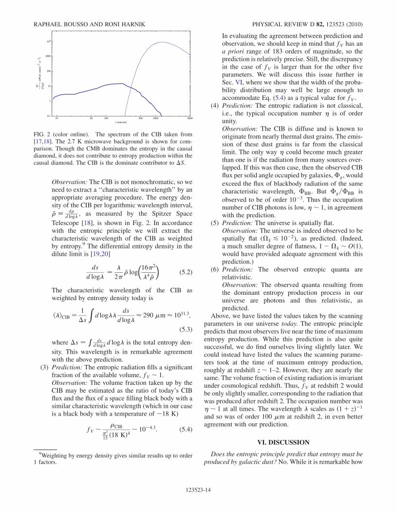
Observation: The CIB is not monochromatic, so weneed to extract a ‘‘characteristic wavelength’’ by anappropriate averaging procedure. The energy den-sity of the CIB per logarithmic wavelength interval,

~� � d�d log� , as measured by the Spitzer Space

Telescope [18], is shown in Fig. 2. In accordancewith the entropic principle we will extract thecharacteristic wavelength of the CIB as weightedby entropy.9 The differential entropy density in thedilute limit is [19,20]

ds

d log�¼ �

2�~� log

�16�2

�4 ~�

�(5.2)

The characteristic wavelength of the CIB asweighted by entropy density today is

h�iCIB ¼ 1

�s

Zd log��

ds

d log�� 290 �m� 1031:3;

(5.3)

where �s ¼ Rds

d log� d log� is the total entropy den-

sity. This wavelength is in remarkable agreementwith the above prediction.

(3) Prediction: The entropic radiation fills a significantfraction of the available volume, fV � 1.Observation: The volume fraction taken up by theCIB may be estimated as the ratio of today’s CIBflux and the flux of a space filling black body with asimilar characteristic wavelength (which in our caseis a black body with a temperature of �18 K)

fV � �CIB

�2

15 ð18 KÞ4 � 10�4:3: (5.4)

In evaluating the agreement between prediction andobservation, we should keep in mind that fV has ana priori range of 183 orders of magnitude, so theprediction is relatively precise. Still, the discrepancyin the case of fV is larger than for the other fiveparameters. We will discuss this issue further inSec. VI, where we show that the width of the proba-bility distribution may well be large enough toaccommodate Eq. (5.4) as a typical value for fV .

(4) Prediction: The entropic radiation is not classical,i.e., the typical occupation number � is of orderunity.Observation: The CIB is diffuse and is known tooriginate from nearly thermal dust grains. The emis-sion of these dust grains is far from the classicallimit. The only way � could become much greaterthan one is if the radiation from many sources over-lapped. If this was then case, then the observed CIBflux per solid angle occupied by galaxies,�g, would

exceed the flux of blackbody radiation of the samecharacteristic wavelength, �BB. But �g=�BB is

observed to be of order 10�3. Thus the occupationnumber of CIB photons is low, �� 1, in agreementwith the prediction.

(5) Prediction: The universe is spatially flat.Observation: The universe is indeed observed to bespatially flat (�k & 10�2), as predicted. (Indeed,a much smaller degree of flatness, 1��k �Oð1Þ,would have provided adequate agreement with thisprediction.)

(6) Prediction: The observed entropic quanta arerelativistic.Observation: The observed quanta resulting fromthe dominant entropy production process in ouruniverse are photons and thus relativistic, aspredicted.

Above, we have listed the values taken by the scanningparameters in our universe today. The entropic principlepredicts that most observers live near the time of maximumentropy production. While this prediction is also quitesuccessful, we do find ourselves living slightly later. Wecould instead have listed the values the scanning parame-ters took at the time of maximum entropy production,roughly at redshift z� 1–2. However, they are nearly thesame. The volume fraction of existing radiation is invariantunder cosmological redshift. Thus, fV at redshift 2 wouldbe only slightly smaller, corresponding to the radiation thatwas produced after redshift 2. The occupation number was�� 1 at all times. The wavelength � scales as ð1þ zÞ�1

and so was of order 100 �m at redshift 2, in even betteragreement with our prediction.

VI. DISCUSSION

Does the entropic principle predict that entropy must beproduced by galactic dust? No. While it is remarkable how

10 50 100 500 1000 50000.1

1

10

100

1000

104

micron

d

dlo

gnW

att

met

er2

sr1

FIG. 2 (color online). The spectrum of the CIB taken from[17,18]. The 2.7 K microwave background is shown for com-parison. Though the CMB dominates the entropy in the causaldiamond, it does not contribute to entropy production within thecausal diamond. The CIB is the dominate contributor to �S.

9Weighting by energy density gives similar results up to order1 factors.


123523-14

many successful, quantitative predictions follow from thesingle assumption of weighting by entropy production, it isimportant to be clear about what we did not predict. By theentropic principle, most observers should find themselvesin an environment that comes close to maximizing entropyproduction. This led us to investigate how entropy produc-tion may be optimized in a Universe with a given cosmo-logical constant. We kept the discussion as general aspossible, making no assumptions about the specific dynam-ics leading to entropy production. Rather, we asked onlyquestions that are well-defined in arbitrary vacua of thelandscape, such as when and at what wavelength the maxi-mum entropy can be produced.

This allowed us to make predictions for six observablequantities, but not for the mechanism by which the entropyis produced. We argued only that observers in any vacuumshould find that there is some mechanism that achievesparameter values close to those derived in Sec. III, andwhich thus comes close to optimizing entropy production.In our universe, this mechanism happens to be the re-radiation of starlight by dust, but this was not one of ourpredictions. It could not possibly have been one, since wedecided from the start to apply the entropic principle to thelandscape as a whole, which meant that such vacuum-specific concepts as ‘‘dust’’ and ‘‘stars’’ had no place inour analysis.

The entropic principle predicts a flat universe. So whoneeds inflation? This question is really the same as theprevious one. The entropic principle tells us that a flatuniverse is more conducive to complex phenomena thana curved one. It does not tell us how a flat universe isdynamically achieved. This is similar to how a more tradi-tional anthropic criterion, the requirement for galaxies,implies an upper bound on curvature. In either case, theargument works only in the context of a landscape thatgives rise to spatially flat pocket universes.

Without a specific mechanism, the only way to obtainflatness would be by sheer chance. This is exponentiallyunlikely; the small prior probability for flatness wouldoverwhelm the entropic weighting favoring flatness.Thus, a dynamical mechanism, such as inflation, is neededto explain how some fraction of vacua in the string land-scape can become spatially flat.

Five out of our six predictions agree perfectly with thedata. How unhappy should we be that one parameter is 4orders of magnitude off? Let us ignore, for a moment, thesuccessful predictions of spatial flatness and of the relativ-istic nature of entropic radiation, which are of a morequalitative nature. Three of the remaining four predictions(the time of entropy production, the typical occupationnumber, and the wavelength) agree with the respectiveobserved values to within less than an order of magnitude.The fraction of volume occupied by the infrared back-ground radiation in our universe, however, is observed tobe fV � 10�4:3; the predicted value is about 1.

A discrepancy of 4 orders of magnitude looks bad untilwe remember that we have identified only the most likelyvalues of parameters, but not the width of the peak aroundthem. Weighting by entropy production comes on top of anunderlying statistical vacuum distribution of the multi-verse. We have assumed that this underlying distributiondoes not grow so strongly towards some other parametervalues as to overwhelm the weight coming from entropyproduction. However, the underlying distribution cansharpen or widen the peak that would naively be obtainedfrom a flat prior over the logarithm of our parameters.In other contexts [21], deviations of order 104 in certainparameter combinations were found to be natural for aplausible range of prior distributions. Thus, the only con-cern is that our predictions may be so uncertain as to bevacuous. However, even a fairly wide peak of 4 orders ofmagnitude in fV (under which the observed value would behighly typical, i.e., in the 1� region) would still constitutea rather restrictive prediction, since fV can vary a prioriover 183 orders of magnitude in vacua with � ¼ �o.In other words, the volume fraction is still remarkablyclose to a special value.In any case, it is best to regard our result as a joint

prediction of (at least) the four parameters (fV , �, tburn,�). The combined discrepancy is only about an order ofmagnitude per parameter, in a four-dimensional logarith-mic parameter space of volume of roughly 63� 61�183� 122� 107. Given the simplicity of the causal en-tropic principle, we regard this as a remarkable success.Doesn’t this result mean that we are atypical at the level

10�5? We have identified the main inefficiency in how ouruniverse produces entropy: the volume fraction occupiedby entropic radiation is only 0:5� 10�4. We have justargued that the probability distribution can be so wide asto make this result quite typical. But how can this be? Arenot observers 104 times more likely to find themselves in auniverse with volume fraction fV ¼ 1=2? This concern isnaive, because prior landscape distributions must be takeninto account. To see this in an explicit example, let usconsider what would happen if we try to design a vacuum‘‘like ours’’ in which the volume fraction occupied byentropic radiation is larger.We would like to hold fixed all other parameters, which

are already (nearly) optimal: the time of dominant entropyproduction, tburn � 10 Gyr, the diluteness of the radiation,�� 1, and the characteristic wavelength, �� 100 �m,the flatness of the universe, and the relativistic nature ofthe entropic radiation. Then the only way to increase thevolume fraction is to burn up a greater fraction of the restmass of the universe.In an optimal Universe all of the rest mass is converted

into entropic radiation. Our Universe is not as energyefficient. Only about a sixth of matter is baryonic. Onlyabout 10% of baryons cooled and fell into stars. Stars burnonly 10% of their baryons. Restricting to baryons that


123523-15

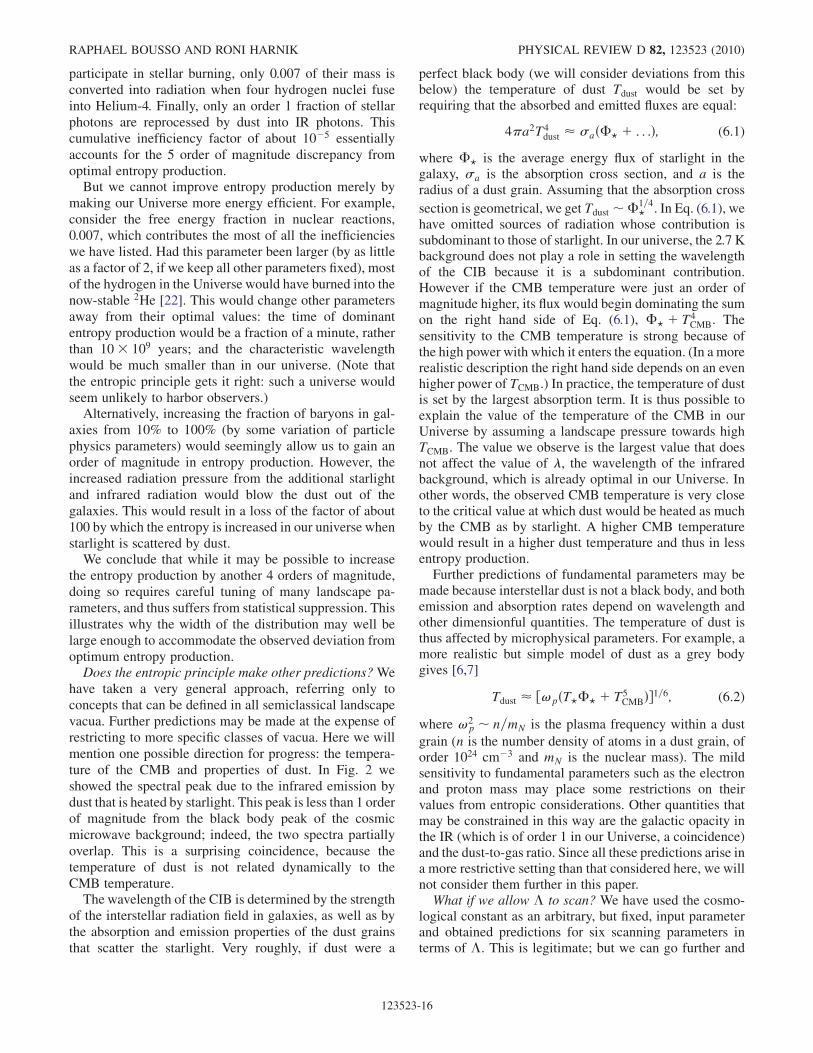
participate in stellar burning, only 0.007 of their mass isconverted into radiation when four hydrogen nuclei fuseinto Helium-4. Finally, only an order 1 fraction of stellarphotons are reprocessed by dust into IR photons. Thiscumulative inefficiency factor of about 10�5 essentiallyaccounts for the 5 order of magnitude discrepancy fromoptimal entropy production.

But we cannot improve entropy production merely bymaking our Universe more energy efficient. For example,consider the free energy fraction in nuclear reactions,0.007, which contributes the most of all the inefficiencieswe have listed. Had this parameter been larger (by as littleas a factor of 2, if we keep all other parameters fixed), mostof the hydrogen in the Universe would have burned into thenow-stable 2He [22]. This would change other parametersaway from their optimal values: the time of dominantentropy production would be a fraction of a minute, ratherthan 10� 109 years; and the characteristic wavelengthwould be much smaller than in our universe. (Note thatthe entropic principle gets it right: such a universe wouldseem unlikely to harbor observers.)

Alternatively, increasing the fraction of baryons in gal-axies from 10% to 100% (by some variation of particlephysics parameters) would seemingly allow us to gain anorder of magnitude in entropy production. However, theincreased radiation pressure from the additional starlightand infrared radiation would blow the dust out of thegalaxies. This would result in a loss of the factor of about100 by which the entropy is increased in our universe whenstarlight is scattered by dust.

We conclude that while it may be possible to increasethe entropy production by another 4 orders of magnitude,doing so requires careful tuning of many landscape pa-rameters, and thus suffers from statistical suppression. Thisillustrates why the width of the distribution may well belarge enough to accommodate the observed deviation fromoptimum entropy production.

Does the entropic principle make other predictions?Wehave taken a very general approach, referring only toconcepts that can be defined in all semiclassical landscapevacua. Further predictions may be made at the expense ofrestricting to more specific classes of vacua. Here we willmention one possible direction for progress: the tempera-ture of the CMB and properties of dust. In Fig. 2 weshowed the spectral peak due to the infrared emission bydust that is heated by starlight. This peak is less than 1 orderof magnitude from the black body peak of the cosmicmicrowave background; indeed, the two spectra partiallyoverlap. This is a surprising coincidence, because thetemperature of dust is not related dynamically to theCMB temperature.

The wavelength of the CIB is determined by the strengthof the interstellar radiation field in galaxies, as well as bythe absorption and emission properties of the dust grainsthat scatter the starlight. Very roughly, if dust were a

perfect black body (we will consider deviations from thisbelow) the temperature of dust Tdust would be set byrequiring that the absorbed and emitted fluxes are equal:

4�a2T4dust � �að�? þ . . .Þ; (6.1)

where �? is the average energy flux of starlight in thegalaxy, �a is the absorption cross section, and a is theradius of a dust grain. Assuming that the absorption cross

section is geometrical, we get Tdust ��1=4? . In Eq. (6.1), we

have omitted sources of radiation whose contribution issubdominant to those of starlight. In our universe, the 2.7 Kbackground does not play a role in setting the wavelengthof the CIB because it is a subdominant contribution.However if the CMB temperature were just an order ofmagnitude higher, its flux would begin dominating the sumon the right hand side of Eq. (6.1), �? þ T4

CMB. The

sensitivity to the CMB temperature is strong because ofthe high power with which it enters the equation. (In a morerealistic description the right hand side depends on an evenhigher power of TCMB.) In practice, the temperature of dustis set by the largest absorption term. It is thus possible toexplain the value of the temperature of the CMB in ourUniverse by assuming a landscape pressure towards highTCMB. The value we observe is the largest value that doesnot affect the value of �, the wavelength of the infraredbackground, which is already optimal in our Universe. Inother words, the observed CMB temperature is very closeto the critical value at which dust would be heated as muchby the CMB as by starlight. A higher CMB temperaturewould result in a higher dust temperature and thus in lessentropy production.Further predictions of fundamental parameters may be

made because interstellar dust is not a black body, and bothemission and absorption rates depend on wavelength andother dimensionful quantities. The temperature of dust isthus affected by microphysical parameters. For example, amore realistic but simple model of dust as a grey bodygives [6,7]

Tdust � ½!pðT?�? þ T5CMBÞ1=6; (6.2)

where !2p � n=mN is the plasma frequency within a dust

grain (n is the number density of atoms in a dust grain, oforder 1024 cm�3 and mN is the nuclear mass). The mildsensitivity to fundamental parameters such as the electronand proton mass may place some restrictions on theirvalues from entropic considerations. Other quantities thatmay be constrained in this way are the galactic opacity inthe IR (which is of order 1 in our Universe, a coincidence)and the dust-to-gas ratio. Since all these predictions arise ina more restrictive setting than that considered here, we willnot consider them further in this paper.What if we allow � to scan? We have used the cosmo-

logical constant as an arbitrary, but fixed, input parameterand obtained predictions for six scanning parameters interms of �. This is legitimate; but we can go further and


123523-16

ask what values of � are most likely to be observed,assuming nothing else. What happens if we allow allparameters to scan, including �?

What happens depends critically on the underlyingprobability distribution in the landscape of vacua. This isreliably known only for � itself: Since � ¼ 0 is not aspecial point from the particle physics point of view,the prior probability distribution is d~p=d� � const forj�j � 1 by Taylor expansion. Combing this with theentropic weighting obtained after integrating out all other

parameters, �S��3=4, and assuming a flat prior on thelogarithm of all other parameters, we obtain10

dp

d�/ �1=4: (6.3)

This would still favor large values of�, suggesting that weare the least complex observers possible. Our intuitionrebels against this conclusion, though we have not founda sharp argument that it conflicts with observation.

However, the conclusion is far from inevitable, since theprior distributions may well be different. We will focus ona particular parameter, the time tburn, when most entropy isproduced (or, via the entropic principle, when observerslive). It may well be easier to produce more entropy at latetimes. In other words, there may be a landscape forcefavoring large values of tburn (or more generally, largevalues of tobs, if we were modelling observers not byentropy production but in some other way). This is simplythe statement that it takes a long time to make complexthings, especially if they emerge from an unguided process.Let us express this assumption as

dp

dtburn/ tburn; (6.4)

where is a positive number of order unity.We have shown in Sec. III that optimizing entropy

production sets tburn ! t�. Thus, after integrating outtburn, the above pressure towards large values of tburn isinherited by t�, adding to the probability distribution

over t� � j�j�1=2. Thus, Eq. (6.3) becomes

dp

d�/ j�jð1=4Þ�ð=2Þ: (6.5)

If > 1=2, which seems to us far from implausible, theprobability distribution favors small values of the cosmo-logical constant.11 In this case, we would find ourselves atthe ‘‘discretuum limit.’’ The cosmological constant we

observe is controlled by the smallest value of j�j in thewhole landscape, which in turn is roughly the inverse of thenumber of vacua with observers.This possibility strikes us as extremely interesting, in

that it relates the observed value of� directly to the size ofthe string landscape. It is particularly intriguing that someestimates of the numberN of metastable vacua have givenlog10N � 500 [1,23]. Note that the number of anthropic

vacua may be a very small fraction (perhaps 10�Oð100Þ of allvacua. So we should not conclude that we live in thevacuum with the smallest cosmological constant; we canconclude only that the value we observe is related to thissmallest value by some factor that captures the rarity ofvacua with particle physics and cosmological parametersthat admit complex phenomena such as observers. Frompurely mathematical facts (the number 500 is related to thenumber of distinct topological cycles in certain manifolds),this could explain the origin of a kind of ur-hierarchy inphysics, from which all other hierarchies may be derivedeither by symmetry arguments of anthropic correlations.Can the entropic principle be improved? We hope so,

and leave this to future work. Clearly, entropy production isan imperfect proxy for observers. It is easy to imagineprocesses that optimize entropy production but are notaccompanied by any kind of complex phenomenon.Worse, such processes may be the norm. For example,one would expect that for every vacuum like ours, withcomplex galaxies, long-lived stars, planets, and organicmolecules, there are many vacua (with the same cosmo-logical constant) in which equal or more entropy is pro-duced by the decay of a single neutrino species with mass3 meV and lifetime 10 Gyr. These vacua should be moreabundant because unlike in our vacuum, the dominantentropy production process would not be predicated onthe complex interplay (and concomitant tuning) of a largenumber of particle physics parameters. Despite the near-maximal entropy production, this process would be veryprimitive, with each neutrino producing a couple ofphotons or other decay products, and no complex struc-tures of any type.This is not necessarily a problem. Our predictions were

successful anyway, because they did not depend on assum-ing that entropy production is sufficient for observers. Butthe entropic principle does assume something stronger thanthe innocuous statement that entropy production is neces-sary: It posits that the number of observers is proportionalto the amount of entropy produced. This is likely to workbest if we average over (i.e., integrate out) most landscapeparameters, as we have done here. In other words, the factthat we considered the whole landscape was actuallybeneficial.In a more restrictive setting, the entropic principle has

greater limitations. For example, if we focussed on a uni-verse like ours except for the value of �, but (unlikeRef. [4]) allowed � to scan over a range large enough to

10This distribution differs from the result of [4] in which dpd� �

const because there we held tburn fixed while only scanning �and here we are letting tburn scan.11The special case ¼ 1=2 leads to a constant probabilitydistribution over logj�j. The conclusions in this case are similarto the case > 1=2, except that our value of � would be relatedonly to the order of magnitude, not to the actual value, of thesmallest j�j in the landscape.


123523-17

include t� � treheat, the probability distribution over �would be dominated by a second peak near �� t�2

reheat

due to the entropy production at reheating. The challenge,then, will be to find a proxy for observers that captures thenotion of ‘‘complexity’’ more reliably, while preservingthe simplicity, generality, and phenomenological successesof the entropic principle. It is possible that some of thecriteria developed in the existing literature on complexitywill be of use here.

ACKNOWLEDGMENTS

We are grateful to M. Arvanitaki, M. Davis, S.Dimopoulos, S. Dubovsky, D. Finkbeiner, B. Freivogel,P. Graham, L. Hall, S. Leichenauer, Y. Nomura, P.Richards, and U. Seljak for discussions. The work ofR. B. was supported by the Berkeley Center forTheoretical Physics, by the National Science Foundationunder Grant No. 08556553, by the Institute for the Physicsand Mathematics of the Universe, by fqxi under GrantNo. RFP2-08-06, and by the U.S. Department of Energyunder Contract No. DE-AC02-05CH11231.

APPENDIX: THE CAUSAL DIAMOND MEASURE

In a universe with at least one metastable de Sittervacuum, inflation is eternal. All events that can happen atall will happen infinitely many times. To define relativeprobabilities, these infinities must be regulated. This is themeasure problem. The landscape of string theory, whichcontains many metastable de Sitter vacua, has focussedrenewed attention on this old problem.

A number of simple measure proposals have been ruledout by showing that they conflict dramatically with obser-vation. Some of the most promising surviving proposalshave been shown to be exactly equivalent due to global-local dualities, or differ only by relatively small factors[13,14,24]. These include the causal diamond and causalpatch measures (with certain simple initial conditions, thelatter is equivalent to the global light-cone time cutoff), aswell as the ‘‘fat geodesic’’ measure (which is equivalent tothe global scale factor time cutoff in regions where thelatter is well-defined). These measures are generally ingood agreement with observation [4,10,24–26].

The causal patch measure [3] restricts attention to thecausal past of a timelike geodesic in the eternally inflatingmultiverse (or equivalently, of the ‘‘endpoint’’ of the geo-desic on the conformal boundary of spacetime). In thispaper, we use the causal diamond measure [4] (see Fig. 3),which is more restrictive. The causal diamond is the inter-section of the causal patch with the causal future of the

event where the geodesic intersects a reheating surface.(The definition has the disadvantage that the term ‘‘reheat-ing surface’’ is not as sharply defined as one would like fora general measure. This limitation can be overcome byusing the apparent horizon measure, which restricts to thespacetime region covered by the union of the expanding(in the past direction) portions of the past light cones of allpoints on the geodesic.)If we had used the causal patch measure instead of the

causal diamond, we would find that entropy production inour universe is dominated by the CMB. In Sec. VI weargued that the decay of a particle is not a form of entropyproduction associated with truly complex phenomena,since the structures involved consist of only a few bitseach and are essentially independent. Thus it is possiblethat this problem can be overcome with an improved proxyfor observers that captures complexity more reliably.Another problem is that for �< 0, the causal patch favorslarge spatial curvature and/or a small magnitude of thecosmological constant [10]. Indeed, the validity of thecausal patch cutoff, or of any related proposals, in non-eternally inflating regions is questionable; this issuemay have to await a better understanding of spacelikesingularities.It is worth emphasizing that the choice of measure is

independent of how we model observers (see, however,footnote 2). The purpose of the measure is to removedivergences, which arise in eternal inflation independentlyof how observers are modeled.

FIG. 3. The causal patch (shaded triangle) is the past of thefuture endpoint of a geodesic (vertical line) in the multiverse.In this paper we use the causal diamond measure. The causaldiamond (dark shaded) is the intersection of the causal patchwith the future of the point B, where the geodesic intersectsa surface of reheating (dashed). A domain wall separatingtwo vacua is also shown (the large wedge that is open at thebottom).


123523-18

[1] R. Bousso and J. Polchinski, J. High Energy Phys. 06(2000) 006.

[2] S. Kachru, R. Kallosh, A. Linde, and S. P. Trivedi, Phys.Rev. D 68, 046005 (2003).

[3] R. Bousso, Phys. Rev. Lett. 97, 191302 (2006).[4] R. Bousso, R. Harnik, G.D. Kribs, and G. Perez, Phys.

Rev. D 76, 043513 (2007).[5] C. Vafa, arXiv:hep-th/0509212.[6] B. T. Draine, arXiv:astro-ph/0304488.[7] C. D. Andriesse, Vistas Astron. 21, 107 (1977).[8] E. Komatsu et al. (WMAP Collaboration),

arXiv:0803.0547.[9] G. ’t Hooft, arXiv:gr-qc/9310026.[10] R. Bousso and S. Leichenauer, Phys. Rev. D 81, 063524

(2010).[11] D. Phillips and A. Albrecht, arXiv:0903.1622.[12] J. Garriga and A. Vilenkin, J. Cosmol. Astropart. Phys. 01

(2009) 021.[13] R. Bousso, Phys. Rev. D 79, 123524 (2009).[14] R. Bousso and I.-S. Yang, Phys. Rev. D 80, 124024 (2009).[15] L.M. Krauss and G.D. Starkman, arXiv:astro-ph/

0404510.

[16] I. Maor, T.W. Kephart, L.M. Krauss, Y. J. Ng, and G.D.Starkman, arXiv:0812.1015.

[17] M.G. Hauser et al., Astrophys. J. 508, 25 (1998); E. Dweket al., arXiv:astro-ph/9806129.

[18] H. Dole et al., Astron. Astrophys. 451, 417 (2006).[19] M. Planck, Ann. Phys. (Leipzig) 309, No. 3, 553

(1901).[20] G. N. Lewis, Proc. Natl. Acad. Sci. U.S.A. 13, No. 5, 307

(1927).[21] R. Bousso, L. J. Hall, and Y. Nomura, Phys. Rev. D 80,

063510 (2009).[22] For a recent analysis see J. MacDonald and D. J. Mullan,

Phys. Rev. D 80, 043507 (2009).[23] F. Denef and M.R. Douglas, J. High Energy Phys. 05

(2004) 072.[24] R. Bousso, B. Freivogel, and I.-S. Yang, Phys. Rev. D 79,

063513 (2009).[25] J.M. Cline, A. R. Frey, and G. Holder, Phys. Rev. D 77,

063520 (2008).[26] B. Bozek, A. J. Albrecht, and D. Phillips, Phys. Rev. D 80,

023527 (2009).


123523-19

http://dx.doi.org/10.1088/1126-6708/2000/06/006

http://dx.doi.org/10.1088/1126-6708/2000/06/006



http://dx.doi.org/10.1103/PhysRevLett.97.191302



http://arXiv.org/abs/hep-th/0509212

http://arXiv.org/abs/astro-ph/0304488

http://dx.doi.org/10.1016/0083-6656(77)90017-4

http://arXiv.org/abs/0803.0547

http://arXiv.org/abs/gr-qc/9310026




http://dx.doi.org/10.1088/1475-7516/2009/01/021

http://dx.doi.org/10.1088/1475-7516/2009/01/021






http://dx.doi.org/10.1086/306379


http://dx.doi.org/10.1051/0004-6361:20054446

http://dx.doi.org/10.1002/andp.19013090310

http://dx.doi.org/10.1002/andp.19013090310

http://dx.doi.org/10.1073/pnas.13.5.307

http://dx.doi.org/10.1073/pnas.13.5.307




http://dx.doi.org/10.1088/1126-6708/2004/05/072

http://dx.doi.org/10.1088/1126-6708/2004/05/072







Entropic landscape

Documents

Transcript of Entropic landscape