Universitat Politècnica de Catalunya (UPC)BarcelonaTech

Facultat d’Informàtica de Barcelona (FIB)

Barcelona Supercomputing Center (BSC-CNS)

Scalability Study of Deep LearningAlgorithms in High Performance

Computer Infrastructures

Francesc Sastre Cabot

Master in Informatics Engineering

Advisor: Jordi Torres i ViñalsUniversitat Politècnica de Catalunya (UPC)

Department of Computer Architecture (DAC)

Co-Advisor: Maurici Yagües GomàBarcelona Supercomputing Center (BSC)

Computer Sciences - Autonomic Systems and e-Business Platforms

April 28, 2017

Abstract

Deep learning algorithms base their success on building high learning capacitymodels with millions of parameters that are tuned in a data-driven fashion.These models are trained by processing millions of examples, so that the de-velopment of more accurate algorithms is usually limited by the throughputof the computing devices on which they are trained.

This project show how the training of a state-of-the-art neural networkfor computer vision can be parallelized on a distributed GPU cluster, Mino-tauro GPU cluster from Barcelona Supercomputing Center with the Tensor-Flow framework.

In this project, two approaches for distributed training are used, the syn-chronous and the mixed-asynchronous. The effect of distributing the trainingprocess is addressed from two different points of view. First, the scalability ofthe task and its performance in the distributed setting are analyzed. Second,the impact of distributed training methods on the final accuracy of the modelsis studied.

The results show an improvement for both focused areas. On one hand,the experiments show promising results in order to train a neural networkfaster. The training time is decreased from 106 hours to 16 hours in mixed-asynchronous and 12 hours in synchronous. On the other hand we can observehow increasing the numbers of GPUs in one node rises the throughput, imagesper second, in a near-linear way. Moreover the accuracy can be maintained,like the one node training, in the synchronous methods.

2

Acknowledgements

I would like to thank my advisor, Jordi Torres, for the great opportunityhe has offered me and for introducing me to the exciting High-PerformanceComputer and Deep Learning worlds, as well his encouraging and enthusiasm.Also, thanks to my co-advisor, Maurici Yagües, for his help, advice, and pa-tience. I also would want to highlight the great job done by the BSC SupportTeam. Thanks to all because without you this project would not have beenpossible.

Thanks to all my colleagues at the Autonomic Systems and e-Business Plat-forms group (BSC) for making an enjoyable working environment, especiallyto Víctor Campos and Míriam Bellver for all things that I have learned fromthem.

I also would render thanks to Alberto, my friend during the degree, themaster, and now at work which without him, none of this would have started.

Last but not least, my special thanks to my family and friends, for theirsupport and comprehension when I have needed it.

4

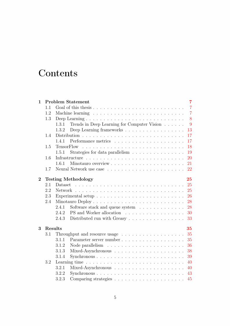
Contents

1 Problem Statement 71.1 Goal of this thesis . . . . . . . . . . . . . . . . . . . . . . . . . . 71.2 Machine learning . . . . . . . . . . . . . . . . . . . . . . . . . . 71.3 Deep Learning . . . . . . . . . . . . . . . . . . . . . . . . . . . . 8

1.3.1 Trends in Deep Learning for Computer Vision . . . . . . 91.3.2 Deep Learning frameworks . . . . . . . . . . . . . . . . . 13

1.4 Distribution . . . . . . . . . . . . . . . . . . . . . . . . . . . . . 171.4.1 Performance metrics . . . . . . . . . . . . . . . . . . . . 17

1.5 TensorFlow . . . . . . . . . . . . . . . . . . . . . . . . . . . . . 181.5.1 Strategies for data parallelism . . . . . . . . . . . . . . . 19

1.6 Infrastructure . . . . . . . . . . . . . . . . . . . . . . . . . . . . 201.6.1 Minotauro overview . . . . . . . . . . . . . . . . . . . . . 21

1.7 Neural Network use case . . . . . . . . . . . . . . . . . . . . . . 22

2 Testing Methodology 252.1 Dataset . . . . . . . . . . . . . . . . . . . . . . . . . . . . . . . 252.2 Network . . . . . . . . . . . . . . . . . . . . . . . . . . . . . . . 252.3 Experimental setup . . . . . . . . . . . . . . . . . . . . . . . . . 262.4 Minotauro Deploy . . . . . . . . . . . . . . . . . . . . . . . . . . 28

2.4.1 Software stack and queue system . . . . . . . . . . . . . 282.4.2 PS and Worker allocation . . . . . . . . . . . . . . . . . 302.4.3 Distributed run with Greasy . . . . . . . . . . . . . . . . 33

3 Results 353.1 Throughput and resource usage . . . . . . . . . . . . . . . . . . 35

3.1.1 Parameter server number . . . . . . . . . . . . . . . . . . 353.1.2 Node parallelism . . . . . . . . . . . . . . . . . . . . . . 363.1.3 Mixed-Asynchronous . . . . . . . . . . . . . . . . . . . . 383.1.4 Synchronous . . . . . . . . . . . . . . . . . . . . . . . . . 39

3.2 Learning time . . . . . . . . . . . . . . . . . . . . . . . . . . . . 403.2.1 Mixed-Asynchronous . . . . . . . . . . . . . . . . . . . . 403.2.2 Synchronous . . . . . . . . . . . . . . . . . . . . . . . . . 433.2.3 Comparing strategies . . . . . . . . . . . . . . . . . . . . 45

5

4 Conclusions 474.1 Project outcomes . . . . . . . . . . . . . . . . . . . . . . . . . . 474.2 Personal outcome . . . . . . . . . . . . . . . . . . . . . . . . . . 494.3 Future work . . . . . . . . . . . . . . . . . . . . . . . . . . . . . 50

Bibliography 53

6

1. Problem Statement

1.1 Goal of this thesis

The aim of this master thesis is to test the scalability of the TensorFlowframework in the Minotauro machine (GPU cluster) at Barcelona Supercom-puting Center (BSC) continuing the work started in the thesis of MauriciYagües [104]. The contents of this thesis may be valuable for the BarcelonaSupercomputing Center in order to define new strategies, new research fieldsand to prove that Deep Learning problems can take advantage of high perfor-mance computers in order to obtain better results in less time.

This document will be focused in three areas: (1) Choose the best configu-ration to distribute the Deep Learning algorithms, (2) study the scalability interms of throughput and (3) the scalability from the learning standpoint.

The introduction of this thesis will introduce the ideas of Machine Learningand Deep Learning, explore different applications of Neural Networks, andshow a brief detail about the most popular Deep Learning frameworks. Also,it will explain the concepts of distribution in Deep Learning , the infrastructureto be used, and the Neural Network use case of this thesis.

1.2 Machine learning

Machine learning (ML) is an Artificial Intelligence subfield that providescomputers with the ability to learn without being explicitly programmed. AMachine Learning algorithm can change its output depending of the data thatit has learned. This kind of algorithms learn data in order to find patternsand build a model to predict and classify items. Machine learning performswell in some scenarios, although there are some cases where it cannot createan accurate model due to the large amount of variations that the problem has.

For example, a classifier of animal pictures. Pictures of same animal canbe much different, different positions, different daylight, different atmosphericconditions, obstructions. A traditional Machine learning algorithm cannot

7

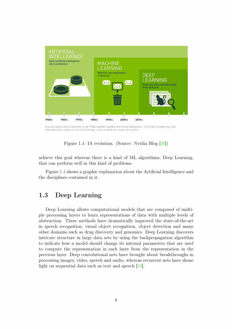
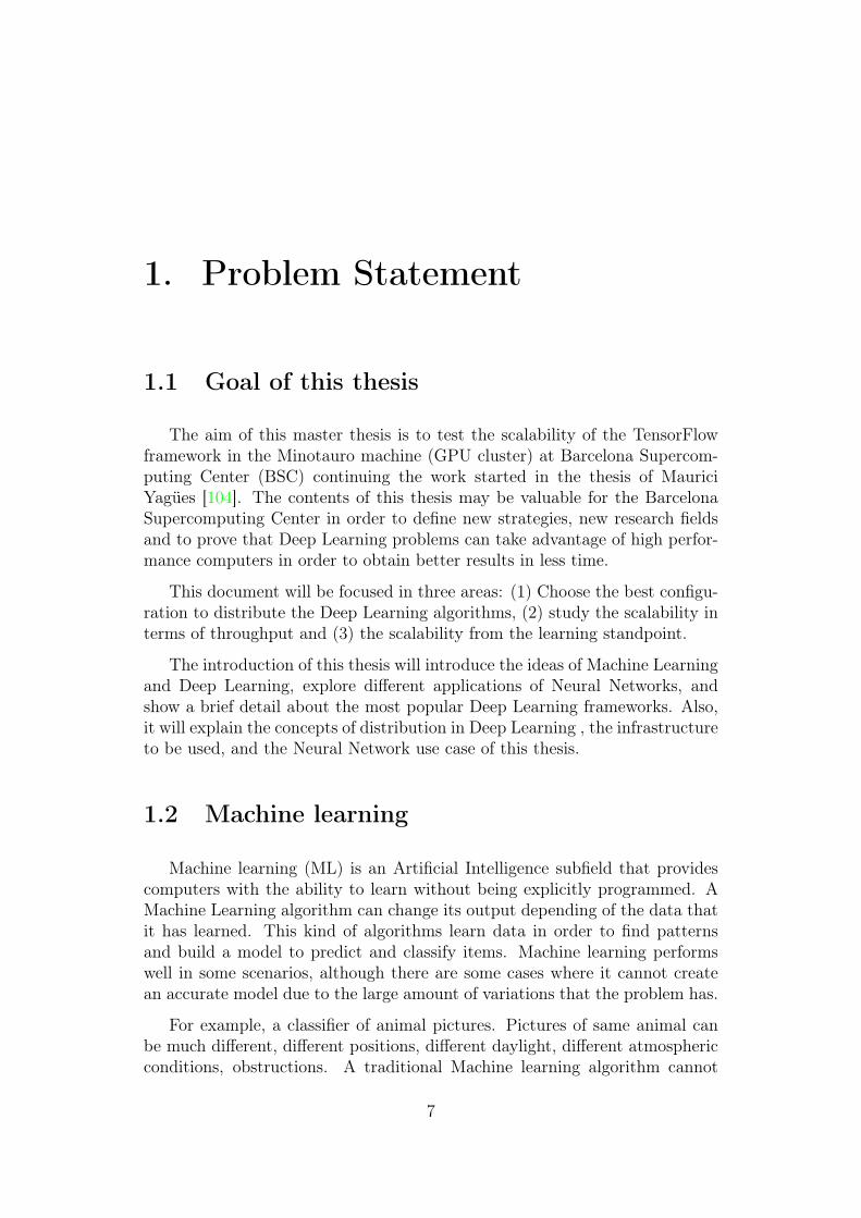
Figure 1.1: IA evolution. (Source: Nvidia Blog [26])

achieve this goal whereas there is a kind of ML algorithms, Deep Learning,that can perform well in this kind of problems.

Figure 1.1 shows a graphic explanation about the Artificial Intelligence andthe disciplines contained in it.

1.3 Deep Learning

Deep Learning allows computational models that are composed of multi-ple processing layers to learn representations of data with multiple levels ofabstraction. These methods have dramatically improved the state-of-the-artin speech recognition, visual object recognition, object detection and manyother domains such as drug discovery and genomics. Deep Learning discoversintricate structure in large data sets by using the backpropagation algorithmto indicate how a model should change its internal parameters that are usedto compute the representation in each layer from the representation in theprevious layer. Deep convolutional nets have brought about breakthroughs inprocessing images, video, speech and audio, whereas recurrent nets have shonelight on sequential data such as text and speech [53].

8

1.3.1 Trends in Deep Learning for Computer Vision

Recently, the fields covered by Deep Learning have increased exponentially.Here, several trends will be explained in order to offer a global vision aboutDeep Learning and how far it reaches. These Deep Learning applications workin a very similar way as the application of this thesis and they could be scaledup as the model of this thesis.

ImageNet classification

ImageNet[31] is an image database organized according to the WordNet1hierarchy. ImageNet aims to populate the majority of the 80,000 synsets ofWordNet with an average of 500-1000 clean and full resolution images. Thiswill result in tens of millions of annotated images organized by the semantichierarchy of WordNet. Figure 1.2 shows an example of Imagenet classification.

Figure 1.2: ImageNet classification. (Source: Alex Krizhevsky et al. [51])

There are several publications about ImageNet classification. AlexNet [51],GoogleNet [91], VGG-Net [86] and Resnet [38] are some of the most used deepmodels to do ImageNet classification. Most Deep Learning frameworks comewith this pre-trained models and they can be used to create new models savingmuch training time.

Object Detection

A simple image classification problem assumes that there is only one targetto classify in the image. Detection problems are about to detect differentobjects in a image and then classify them individually. There are severalmethods based on deep neural nets to realize the classification.

1WordNet website (https://wordnet.princeton.edu/)

9

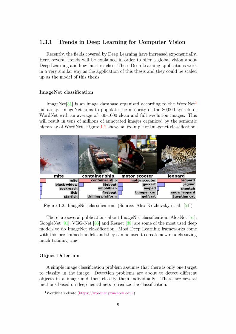
Figure 1.3: Object detection and classification. Images with regions and clas-sifications. (Source: Shaoqing Ren et al. [79])

Some of these methods use a two stage procedure to detect and classifyas R-CNN [36], Fast R-CNN [35], Faster R-CNN [79] or R-FCN [28]. In thetwo stage methods, the image goes through a network in order extract featuresand at some point (layer), the detector finds the regions on the image wherethere are objects. These regions are cut in the image and sent to classifyusing a neural net. The network can be another one, the same used for theobject detection, or even the classification can continue at the same layer ofthe detection. Figure 1.3 shows examples of object detection.

On the other hand there are methods that can do all in one stage, theycan detect and classify going through the network once. Some examples areYOLO [78] or SSD [56].

An important point for object detection is performance for real-time de-tection, for mobile or embedded applications. Jonathan Huang et al. in"Speed/accuracy trade-offs for modern convolutional object detectors" [40]compares the different object detectors using different neural nets in terms ofspeed, memory or accuracy.

Edge Detection

The edge detection problem with deep neural networks is strongly related tothe object detection problem. Edge detection is a way for segmentation, imageclassification and object tracking. Saining Xie et al. [102], Gedas Bertasiuset al. with DeepEdge [9] and Wei Shen et al. with DeepContour [83] try toaddress the problem with different strategies. Figure 1.4 shows an example ofedge detection using deep neural networks.

10

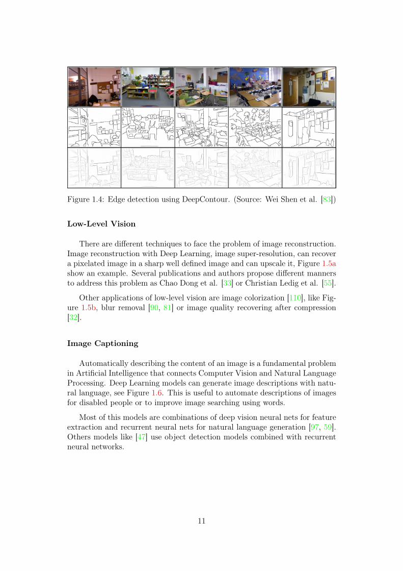
Figure 1.4: Edge detection using DeepContour. (Source: Wei Shen et al. [83])

Low-Level Vision

There are different techniques to face the problem of image reconstruction.Image reconstruction with Deep Learning, image super-resolution, can recovera pixelated image in a sharp well defined image and can upscale it, Figure 1.5ashow an example. Several publications and authors propose different mannersto address this problem as Chao Dong et al. [33] or Christian Ledig et al. [55].

Other applications of low-level vision are image colorization [110], like Fig-ure 1.5b, blur removal [90, 81] or image quality recovering after compression[32].

Image Captioning

Automatically describing the content of an image is a fundamental problemin Artificial Intelligence that connects Computer Vision and Natural LanguageProcessing. Deep Learning models can generate image descriptions with natu-ral language, see Figure 1.6. This is useful to automate descriptions of imagesfor disabled people or to improve image searching using words.

Most of this models are combinations of deep vision neural nets for featureextraction and recurrent neural nets for natural language generation [97, 59].Others models like [47] use object detection models combined with recurrentneural networks.

11

(a) Super Resolution application. (Source: Christian Ledig et al. [55])

(b) Image Colorization. (Source: Richard Zhang et al. [110])

Figure 1.5: Low-level vision applications.

Figure 1.6: Images with captions. (Source: Andrej Karpathy et al. [47])

12

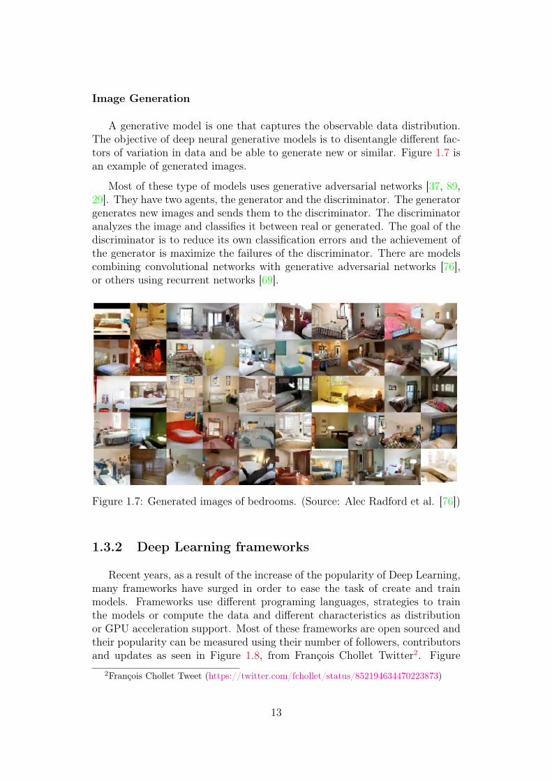
Image Generation

A generative model is one that captures the observable data distribution.The objective of deep neural generative models is to disentangle different fac-tors of variation in data and be able to generate new or similar. Figure 1.7 isan example of generated images.

Most of these type of models uses generative adversarial networks [37, 89,29]. They have two agents, the generator and the discriminator. The generatorgenerates new images and sends them to the discriminator. The discriminatoranalyzes the image and classifies it between real or generated. The goal of thediscriminator is to reduce its own classification errors and the achievement ofthe generator is maximize the failures of the discriminator. There are modelscombining convolutional networks with generative adversarial networks [76],or others using recurrent networks [69].

Figure 1.7: Generated images of bedrooms. (Source: Alec Radford et al. [76])

1.3.2 Deep Learning frameworks

Recent years, as a result of the increase of the popularity of Deep Learning,many frameworks have surged in order to ease the task of create and trainmodels. Frameworks use different programing languages, strategies to trainthe models or compute the data and different characteristics as distributionor GPU acceleration support. Most of these frameworks are open sourced andtheir popularity can be measured using their number of followers, contributorsand updates as seen in Figure 1.8, from François Chollet Twitter2. Figure

2François Chollet Tweet (https://twitter.com/fchollet/status/852194634470223873)

13

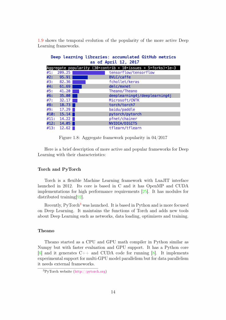
1.9 shows the temporal evolution of the popularity of the more active DeepLearning frameworks.

Figure 1.8: Aggregate framework popularity in 04/2017

Here is a brief description of more active and popular frameworks for DeepLearning with their characteristics:

Torch and PyTorch

Torch is a flexible Machine Learning framework with LuaJIT interfacelaunched in 2012. Its core is based in C and it has OpenMP and CUDAimplementations for high performance requirements [25]. It has modules fordistributed training[92].

Recently, PyTorch3 was launched. It is based in Python and is more focusedon Deep Learning. It maintains the functions of Torch and adds new toolsabout Deep Learning such as networks, data loading, optimizers and training.

Theano

Theano started as a CPU and GPU math compiler in Python similar asNumpy but with faster evaluation and GPU support. It has a Python core[6] and it generates C++ and CUDA code for running [8]. It implementsexperimental support for multi-GPU model parallelism but for data parallelismit needs external frameworks.

3PyTorch website (http://pytorch.org)

14

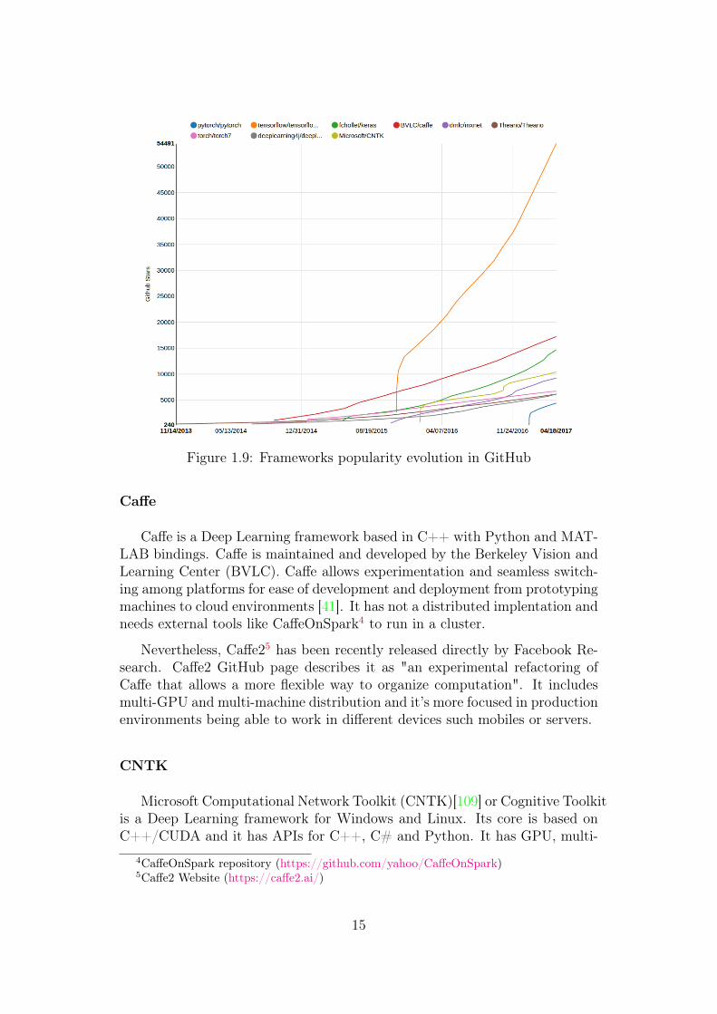
Figure 1.9: Frameworks popularity evolution in GitHub

Caffe

Caffe is a Deep Learning framework based in C++ with Python and MAT-LAB bindings. Caffe is maintained and developed by the Berkeley Vision andLearning Center (BVLC). Caffe allows experimentation and seamless switch-ing among platforms for ease of development and deployment from prototypingmachines to cloud environments [41]. It has not a distributed implentation andneeds external tools like CaffeOnSpark4 to run in a cluster.

Nevertheless, Caffe25 has been recently released directly by Facebook Re-search. Caffe2 GitHub page describes it as "an experimental refactoring ofCaffe that allows a more flexible way to organize computation". It includesmulti-GPU and multi-machine distribution and it’s more focused in productionenvironments being able to work in different devices such mobiles or servers.

CNTK

Microsoft Computational Network Toolkit (CNTK)[109] or Cognitive Toolkitis a Deep Learning framework for Windows and Linux. Its core is based onC++/CUDA and it has APIs for C++, C# and Python. It has GPU, multi-

4CaffeOnSpark repository (https://github.com/yahoo/CaffeOnSpark)5Caffe2 Website (https://caffe2.ai/)

15

GPU and distributed training support. CNTK uses graph computation andallows to easily realize and combine popular model types such as feed-forwardDNNs, convolutional nets (CNNs), and recurrent networks (RNNs/LSTMs).It implements stochastic gradient descent (SGD, error backpropagation) andlearning with automatic differentiation. CNTK has been available under anopen-source license since April 2015.

Microsoft offers CNTK as a service in the Azure Platform6 with GPUinstances.

MXNET

MXNET is a multi-language framework for Machine Learning. It has aC++ core and Python, R, C++ and Julia bindings. It is compatible with CPUand GPUs and natively supports GPU parallelism and distributed execution.MXNET supports declarative and imperative execution and permits the userto choose which want to use. MXNet is computation and memory efficientand runs on various heterogeneous systems, ranging from mobile devices todistributed GPU clusters [22].

deeplearning4j

Deeplearning4j7 is an open-source, distributed deep-learning library writtenfor Java and Scala. Integrated with Hadoop and Spark, DL4J is designed tobe used in business environments on distributed GPUs and CPUs. Its coreis written in C/C++/CUDA and has a Python API using Keras. It usesSpark/Hadoop for the distribution, it is compatible with multi-GPU and itcan run in Amazon AWS Elastic Map Reduce8.

Keras

Keras is a high-level neural networks API, written in Python and capableof running on top of either TensorFlow[1, 2] or Theano[8]. The user can changethe backend (TF/Theano) without changing the code. The Keras code can bemixed with the code of the backend. Keras uses the different characteristicsoffered by the available backends and it is compatible with multi-GPU anddistributed run.

6Azure Deep Learning toolkit for Data Science VM website(https://azuremarketplace.microsoft.com/en-us/marketplace/apps/microsoft-ads.dsvm-deep-learning)

7deeplearning4j website (https://deeplearning4j.org/)8Amazon AWS Elastic Map Reduce website (https://aws.amazon.com/emr/)

16

1.4 Distribution

The main idea behind this computing paradigm is to run tasks concurrentlyinstead of serially, as it would happen in a single machine. To achieve this,there are two principal implementations, and it will depend on the needs ofthe application to know which one will perform better, or even if a mix of bothapproaches can increase the performance.

Data parallelism

In this mode, the training data is divided into multiple subsets, and eachone of them is run on the same replicated model in a different node (workernodes). These will need to synchronize the model parameters (or its gradients)at the end of the batch computation to ensure they are training a consistentmodel. This is straightforward for Machine Learning applications that useinput data as a batch, and the dataset can be partitioned both rowwise (in-stances) and columnwise (features).

Some interesting properties of this setting is that it will scale with theamount of data available and it speeds up the rate at which the entire datasetcontributes to the optimization [71]. Also, it requires less communication be-tween nodes, as it benefits from high amount of computations per weight [50].On the other hand, the model has to entirely fit on each node [27], and it ismainly used for speeding computation of convolutional neural networks withlarge datasets.

Model parallelism

In this case, the model will be segmented into different parts that can runconcurrently, and each one will run on the same data in different nodes. Thescalability of this method depends on the degree of task parallelization of thealgorithm, and it is more complex to implement than the previous one. Itmay decrease the communication needs, as workers need only to synchronizethe shared parameters (usually once for each forward or backward-propagationstep) and works well for GPUs in a single server that share a high speed bus[24]. It can be used with larger models as hardware constraints per node areno more a limitation, but is highly vulnerable to worker failures.

1.4.1 Performance metrics

The term performance in these systems has a double interpretation. Onone hand it refers to the predictive accuracy of the model, and on the other to

17

the computational speed of the process. The first metric is independent of theplatform and is the performance metric to compare multiple models, whereasthe second depends on the platform on which the model is deployed and ismainly measured by metrics such as:

• Speedup: ratio of solution time for the sequential algorithms versus itsparallel counterpart

• Efficiency: ratio of speedup to the number of CPUs / GPUs or nodes

• Scalability: efficiency as a function of an increasing number of CPUs /GPUs or nodes

Some of this metrics will be highly dependent on the cluster configuration,the type of network used and the efficiency of the framework using the librariesand managing resources.

1.5 TensorFlow

TensorFlow is a Machine Learning system that operates at large scale andin heterogeneous environments. TensorFlow uses dataflow graphs to representcomputation, shared state, and the operations that mutate that state. It mapsthe nodes of a dataflow graph across many machines in a cluster, and withina machine across multiple computational devices, including multicore CPUs,general purpose GPUs, and custom designed ASICs known as Tensor Pro-cessing Units (TPUs [4]). This architecture gives flexibility to the applicationdeveloper: whereas in previous “parameter server” designs the management ofshared state is built into the system, TensorFlow enables developers to exper-iment with novel optimizations and training algorithms.

The system is flexible and can be used to express a wide variety of algo-rithms, including training and inference algorithms for deep neural networkmodels, and it has been used for conducting research and for deploying Ma-chine Learning systems into production [1, 2].

TensorFlow has Python, Java, Go and C++ bindings and it supports dis-tributed traning using model parallelism and data parallelism. This frameworkis maintained by Google and it has a great support from the community, seeFigures 1.8 and 1.9. Tensorflow has been chosen for this project due to the flex-ibility that it can offer and the awesome support showed on recent years. Lotsof projects and companies have started to migrate from another frameworkssuch Caffe or Theano to Tensorflow.

TensorFlow also includes Tensorboard, see Figure 1.10. Tensorboard isused to visualize the TensorFlow graph, plot quantitative metrics about the

18

execution of the graph like accuracy or loss, and show additional data likeimages, videos or audios.

The first stable release of Tensorflow was released in February 2017. Thisnew version starts a long term support with the promise of maintaining thecompatibility among the different minor versions of this major version. Ten-sorFlow will include the Keras library, see Section 1.3.2, inside the core ofthe framework. With Keras, Tensorflow will decrease its learning curve andattract more developers to the platform.

Figure 1.10: Tensorboard example. (Source: tensorflow.org)

1.5.1 Strategies for data parallelism

There are two types of processes involved in distributed TensorFlow. First,the worker processes, in charge of the computation using GPUs, CPUs and/orTPUs. On the other hand there is the parameter server (PS), this kind ofprocess receives the model updates from the workers, processes them and sendsa new model to the workers.

There are different strategies in order to do data parallelism in TensorFlow.The distinctness is focused in the way to merge the gradients between differentworkers. Chen et al. [19, 20] compare the strategies using a very large numberof workers without focusing in efficiency terms.

Synchronous mode: In this case, the PS waits until all worker nodeshave computed the gradients with respect to their data batches. Once thegradients are received by the PS, they are applied to the current weights andthe updated model is sent back to all the worker nodes. This method is asfast as the slowest node, as no updates are performed until all worker nodesfinish the computation, and may suffer from unbalanced network speeds when

19

(a) Asynchronous replication (b) Synchronous replica-tion

(c) Synchronous withbackup workers

Figure 1.11: Strategies for data parallelism. (Source: Abadi et al. [2])

the cluster is shared with other users. However, faster convergence is achievedas more accurate gradient estimations are obtained. Authors in [20] presentan alternative strategy for alleviating the slowest worker update problem byusing backup workers, as Figure 1.11c.

Asynchronous mode: every time the PS receives the gradients from aworker, the model parameters are updated. Despite delivering an enhancedthroughput when compared to its synchronous counterpart, every worker maybe operating on a slightly different version of the model, thus providing poorergradient estimations. As a result, more iterations are required until conver-gence due to the stale gradient updates. Increasing the number of workersmay result in a throughput bottleneck by the communication with the PS, inwhich case more PS need to be added.

Mixed mode: mixed mode appears as a trade-off between adequate batchsize and throughput by performing asynchronous updates on the model param-eters, but using synchronously averaged gradients coming from subgroups ofworkers. Larger learning rates can be used thanks to the increased batchsize, leading to a faster convergence, while reaching throughput rates close tothose in the asynchronous mode. This strategy also reduces communication ascompared to the pure asynchronous mode.

1.6 Infrastructure

BSC-CNS (Barcelona Supercomputing Center – Centro Nacional de Su-percomputación) is the National Supercomputing Facility in Spain and wasofficially constituted in April 2005. BSC-CNS manages MareNostrum, one ofthe most powerful supercomputers in Europe. The mission of BSC-CNS is toinvestigate, develop and manage information technology in order to facilitatescientific progress. With this aim, special dedication has been taken to areassuch as Computer Sciences, Life Sciences, Earth Sciences and ComputationalApplications in Science and Engineering.

All these activities are complementary to each other and very tightly re-

20

lated. In this way, a multidisciplinary loop is set up: “our exposure to industrialand non-computer science academic practices improves our understanding ofthe needs and helps us focusing our basic research towards improving thosepractices. The result is very positive both for our research work as well as forimproving the way we service our society” [12].

BSC-CNS also has other High Performance Computing (HPC) facilities, asthe NVIDIA GPU Cluster Minotauro that is the one used for this project.

1.6.1 Minotauro overview

Minotauro is a heterogeneous cluster with 2 configurations [13]:

• 61 Bull B505 blades, each blade with the following technical character-istics:

– 2 Intel E5649 (6-Core) processor at 2.53 GHz

– 2 M2090 NVIDIA GPU Cards

– 24 GB of main memory

– Peak Performance: 88.60 TFlops

– 250 GB SSD (Solid State Disk) as local storage

– 2 Infiniband QDR (40 Gbit each) to a non-blocking network

– 14 links of 10 GbitEth to connect to BSC GPFS Storage

• 39 bullx R421-E4 servers, each server with:

– 2 Intel Xeon E5-2630 v3 (Haswell) 8-core processors, (each core at2.4 GHz,and with 20MB L3 cache)

– 2 K80 NVIDIA GPU Cards

– 128 GB of Main memory, distributed in 8 DIMMs of 16 GB - DDR4@ 2133 MHz - ECC SDRAM

– Peak Performance: 250.94 TFlops

– 120 GB SSD (Solid State Disk) as local storage

– 1 PCIe 3.0 x8 8GT/s, Mellanox ConnectXR - 3FDR 56 Gbit

– 4 Gigabit Ethernet ports

The operating system is RedHat Linux 6.7 for both configurations. TheTensorFlow installation is working only on the servers with the NVIDIA K80because the M2090 NVIDIA GPU cards do not have the minimum requiredsoftware specifications TensorFlow demands.

21

Each one of the NVIDIA K80s contain two K40 chips in a single PCB with12 GB GDDR5, so we physically have only two GPUs in each server, but areseen as 4 different cards by the software, see Figure 1.12.

K80 K80

/gpu:0 /gpu:2

/gpu:3/gpu:1

/cpu:1/cpu:0

Figure 1.12: Schema of the hardware in a Minotauro node. (Source: MauriciYagües [104])

1.7 Neural Network use case

Affective Computing [74] has recently garnered much research attention.Machines that are able to understand and convey subjectivity and affect wouldlead to a better human-computer interaction that is key in some fields such asrobotics or medicine. Despite the success in some constrained environmentssuch as emotional understanding of facial expressions [60], automated affectunderstanding in unconstrained domains remains an open challenge which isstill far from other tasks where machines are approaching or have even sur-passed human performance. In this work, we will focus on the detection ofAdjective Noun Pairs (ANPs) using a large-scale image dataset collected fromFlickr [46]. These mid-level representations, which are a rising approach forovercoming the affective gap between low level image features and high levelaffect semantics, can then be used to train accurate models for visual senti-ment analysis or visual emotion prediction. Figure 1.13 shows a brief detailhow the proposed structure works.

22

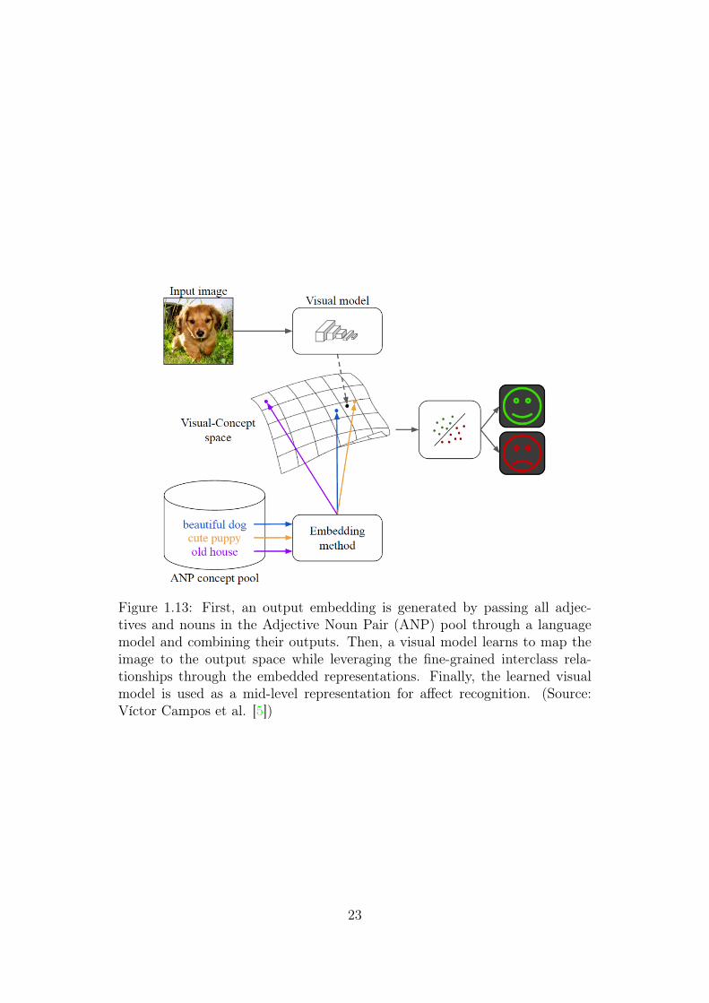
Figure 1.13: First, an output embedding is generated by passing all adjec-tives and nouns in the Adjective Noun Pair (ANP) pool through a languagemodel and combining their outputs. Then, a visual model learns to map theimage to the output space while leveraging the fine-grained interclass rela-tionships through the embedded representations. Finally, the learned visualmodel is used as a mid-level representation for affect recognition. (Source:Víctor Campos et al. [5])

23

24

2. Testing Methodology

2.1 Dataset

Adjective Noun Pairs (ANPs) are powerful mid-level representations [11]that can be used for affect related tasks such as visual sentiment analysis oremotion recognition. A large-scale ANP ontology for 12 different languages,namely Multilingual Visual Sentiment Ontology (MVSO), was collected byJou et al. [46] following a model derived from psychology studies, Plutchick’sWheel of Emotions [75]. The noun component in an ANP can be understoodto ground the visual appearance of the entity, whereas the adjective polarizesthe content towards a positive or negative sentiment, or emotion [46]. Theseproperties try to bridge the affective gap between low level image featuresand high level affective semantics, which goes far beyond recognizing the mainobject in an image. Whereas a traditional object classification algorithm mayrecognize a baby in an image, a finer-grained classification such as happy baby orcrying baby is usually needed to fully understand the affective content conveyedin the image. Capturing the sophisticated differences between ANPs posesa challenging task that requires from high capacity models and large-scaleannotated datasets.

The experiments with the subset of the English partition of MVSO, thetag-restricted subset, which contains over 1.2M samples covering 1,200 differentANPs. Since images in MVSO were downloaded from Flickr and automaticallyannotated using their metadata, such annotations have to be considered asweak labels, i.e. some labels may not match the real content of the images. Thetag-pool subset contains those samples for which the annotation was obtainedfrom the tags in Flickr instead of other metadata, so that annotations are morelikely to match the real ground truth.

2.2 Network

Since the first successful application of Convolutional Neural Nets (CNNs)to large-scale visual recognition, the design of improved architectures for im-

25

proved classification performance has focused on increasing the depth, i.e. thenumber of layers, while keeping or even reducing the number of trainable pa-rameters. This trend can be seen when comparing the 8 layers in AlexNet [51],the first CNN-based method to win the Image Large Scale Visual RecognitionChallenge (ILSVRC) in 2012, with the dozens, or even hundreds, of layers inResidual Nets (ResNets) [38]. Despite the huge increase in the overall depth,a ResNet with 50 layers has roughly half the parameters in AlexNet. However,the impact of an increased depth is more notorious in the memory footprint ofdeeper architectures, which store more intermediate results coming from theoutput of each single layer, thus benefiting from multi-GPU setups that allowthe use of larger batch sizes1.

The ResNet50 CNN [38] is used on the experiments, an architecture with50 layers that maps a 224 × 224 × 3 input image to a 1,200-dimensional vec-tor representing a probability distribution over the ANP classes in the dataset.Overall, the model contains over 25×106 single-precision floating-point param-eters involved in over 4 × 109 floating-point operations that are tuned duringtraining. It is important to notice that the more computationally demanding aCNN is, the larger the gains of a distributed training due to the amount of timespent doing parallel computations with respect to the added communicationoverhead.

Cross-entropy2 between the output of the CNN and the ground truth,i.e. the real class distribution, is used as loss function together with an L2regularization3 term with a weight decay rate of 10−4. The parameters in themodel are tuned to minimize the former cost objective using batch gradientdescent.

2.3 Experimental setup

The experiments are evaluated in a GPU cluster, where each node isequipped with 2 NVIDIA Kepler K80 dual GPU cards, 2 Intel Xeon E5-26308-core processors and 128GB of RAM. Inter-node communication is performedtrough a 56Gb/s InfiniBand network. The CNN architectures and their train-ing are implemented with TensorFlow4, running on CUDA and using cuDNNprimitives for improved performance. Since the training process needs to be

1The batch size is the number of elements that are processed in one iteration of training.The more deep is the network, the more memory is needed and the batch size has to decreaseto fit in the GPU memory, but, if several GPUs are used the batch size can be smaller ineach GPU but in total more elements are processed.

2 CS231n Convolutional Neural Networks for Visual Recognition. Stanford Course(http://cs231n.github.io/linear-classify/)

3See footnote 24TensorFlow website (https://www.tensorflow.org/)

26

submitted through Slurm Workload Manager, task distribution and communi-cation between nodes is achieved with Greasy [93].

(a) Software stack used in theasynchronous setup

(b) Software stack used in the syn-chronous setup

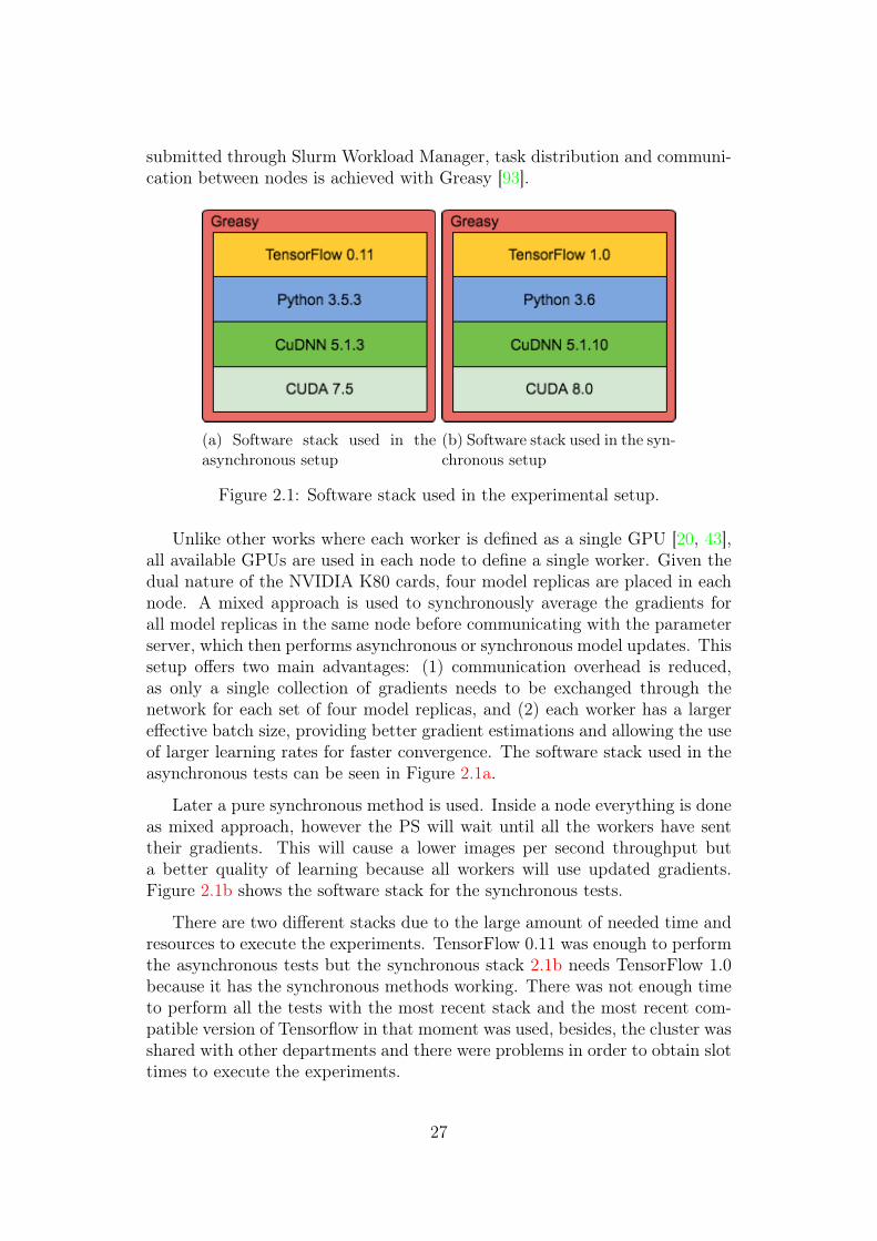
Figure 2.1: Software stack used in the experimental setup.

Unlike other works where each worker is defined as a single GPU [20, 43],all available GPUs are used in each node to define a single worker. Given thedual nature of the NVIDIA K80 cards, four model replicas are placed in eachnode. A mixed approach is used to synchronously average the gradients forall model replicas in the same node before communicating with the parameterserver, which then performs asynchronous or synchronous model updates. Thissetup offers two main advantages: (1) communication overhead is reduced,as only a single collection of gradients needs to be exchanged through thenetwork for each set of four model replicas, and (2) each worker has a largereffective batch size, providing better gradient estimations and allowing the useof larger learning rates for faster convergence. The software stack used in theasynchronous tests can be seen in Figure 2.1a.

Later a pure synchronous method is used. Inside a node everything is doneas mixed approach, however the PS will wait until all the workers have senttheir gradients. This will cause a lower images per second throughput buta better quality of learning because all workers will use updated gradients.Figure 2.1b shows the software stack for the synchronous tests.

There are two different stacks due to the large amount of needed time andresources to execute the experiments. TensorFlow 0.11 was enough to performthe asynchronous tests but the synchronous stack 2.1b needs TensorFlow 1.0because it has the synchronous methods working. There was not enough timeto perform all the tests with the most recent stack and the most recent com-patible version of Tensorflow in that moment was used, besides, the cluster wasshared with other departments and there were problems in order to obtain slottimes to execute the experiments.

27

The loss function5 is minimized using RMSProp [95] per-parameter adap-tive learning rate as optimization method with a learning rate of 0.1, decay of0.9 and ε = 1.0. Each worker has an effective batch size of 128 samples, i.e. 32images are processed at a time by each GPU. To prevent overfitting, data aug-mentation consisting in random crops and/or horizontal flips is asynchronouslyperformed on CPU while previous batches are processed by the GPUs. TheCNN weights are initialized using a model pre-trained6 on ILSVRC [31], prac-tice that has been proven beneficial even when training on large-scale datasets[105].

Previous publications on distributed training with TensorFlow [2, 20] tendto use different server configurations for worker and PS tasks. Given that a PSonly stores and updates the model and there is no need for GPU computations,CPU-only servers are used for this task. On the other hand, most of the workerjob involves matrix computations, for which servers equipped with GPUs areused. All nodes in the cluster used in these experiments are GPU equippednodes, which means that placing PS and workers in different nodes wouldresult in under-utilization of GPU resources. The impact of sharing resourcesbetween PS and workers as compared to the former configuration and whetherthis setup is suitable for a homogeneous cluster where all nodes are equippedwith GPU cards will be studied.

2.4 Minotauro Deploy

2.4.1 Software stack and queue system

MinoTauro uses the GPFS file system, which is shared with MareNostrum.Thanks to this, all nodes of MinoTauro have access to the same files. All thesoftware is allocated in the GPFS system and is also common in all nodes,there are two software folders, the general folder and the K80 folder, the lastfolder contains all the software compiled for the NVIDIA K80 GPUs [13].

MinoTauro comes with a software stack, this software is static and the userscannot modify it. If a user needs a new software, a modification or an update ofan existent software has to request a petition to the BSC-CNS support center.This is the used part of the software stack in this project:

• TensorFlow 0.117: The first version of TensorFlow used in this project.This version has a lot of bug fixes, improvements and new abstraction

5The loss function calculates the difference between the input training example and itsexpected output.

6Pre-training a model is a habitual technique. A pre-trained model, is a model initializedwith the weights resulted from the training with another dataset.

7GitHub release 0.11 https://github.com/tensorflow/tensorflow/releases/tag/v0.11.0rc0

28

layer, TF-Slim, that allows to do some operations more easily.

• TensorFlow 1.08: The second release of TensorFlow used in this project.This version is the first major version of Tensorflow, it establishes a con-sistent API and ensures that the new changes will not break backwardscompatibility unlike the 0.x versions. It provides new abstractions fordistributed training and an improved synchronous training.

• Python 3.5.2/3.6: The Python version installed in the K80 nodes. Itcomes with all required packages by TensorFlow. The 0.11 version usesPython 3.5.2 and the 1.0 version uses Python 3.6.

• CUDA 7.5/8.0: CUDA is a parallel computing platform and program-ming model created by NVIDIA. It enables dramatic increases in com-puting performance by harnessing the power of the GPU [67]. This isrequired to use GPUs with TensorFlow.

• cuDNN 5.1.3/5.1.10: The NVIDIA CUDA Deep Neural Network li-brary is a GPU-accelerated library of primitives for deep neural net-works. cuDNN provides highly tuned implementations for standard rou-tines such as forward and backward convolution, pooling, normalization,and activation layers [23].

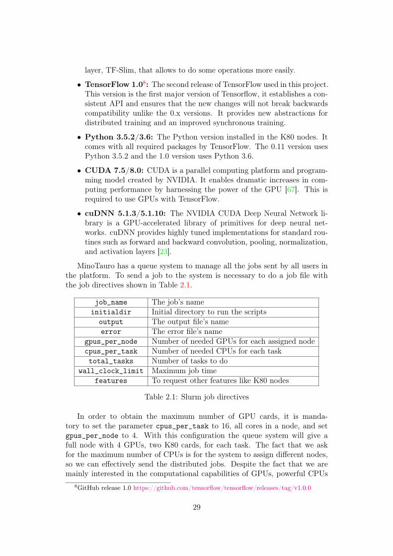
MinoTauro has a queue system to manage all the jobs sent by all users inthe platform. To send a job to the system is necessary to do a job file withthe job directives shown in Table 2.1.

job_name The job’s nameinitialdir Initial directory to run the scripts

output The output file’s nameerror The error file’s name

gpus_per_node Number of needed GPUs for each assigned nodecpus_per_task Number of needed CPUs for each tasktotal_tasks Number of tasks to do

wall_clock_limit Maximum job timefeatures To request other features like K80 nodes

Table 2.1: Slurm job directives

In order to obtain the maximum number of GPU cards, it is manda-tory to set the parameter cpus_per_task to 16, all cores in a node, and setgpus_per_node to 4. With this configuration the queue system will give afull node with 4 GPUs, two K80 cards, for each task. The fact that we askfor the maximum number of CPUs is for the system to assign different nodes,so we can effectively send the distributed jobs. Despite the fact that we aremainly interested in the computational capabilities of GPUs, powerful CPUs

8GitHub release 1.0 https://github.com/tensorflow/tensorflow/releases/tag/v1.0.0

29

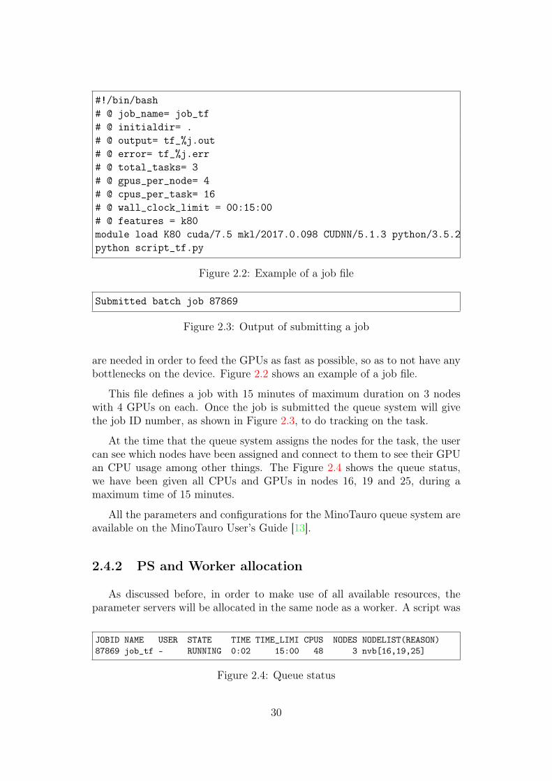
#!/bin/bash# @ job_name= job_tf# @ initialdir= .# @ output= tf_%j.out# @ error= tf_%j.err# @ total_tasks= 3# @ gpus_per_node= 4# @ cpus_per_task= 16# @ wall_clock_limit = 00:15:00# @ features = k80module load K80 cuda/7.5 mkl/2017.0.098 CUDNN/5.1.3 python/3.5.2python script_tf.py

Figure 2.2: Example of a job file

Submitted batch job 87869

Figure 2.3: Output of submitting a job

are needed in order to feed the GPUs as fast as possible, so as to not have anybottlenecks on the device. Figure 2.2 shows an example of a job file.

This file defines a job with 15 minutes of maximum duration on 3 nodeswith 4 GPUs on each. Once the job is submitted the queue system will givethe job ID number, as shown in Figure 2.3, to do tracking on the task.

At the time that the queue system assigns the nodes for the task, the usercan see which nodes have been assigned and connect to them to see their GPUan CPU usage among other things. The Figure 2.4 shows the queue status,we have been given all CPUs and GPUs in nodes 16, 19 and 25, during amaximum time of 15 minutes.

All the parameters and configurations for the MinoTauro queue system areavailable on the MinoTauro User’s Guide [13].

2.4.2 PS and Worker allocation

As discussed before, in order to make use of all available resources, theparameter servers will be allocated in the same node as a worker. A script was

JOBID NAME USER STATE TIME TIME_LIMI CPUS NODES NODELIST(REASON)87869 job_tf - RUNNING 0:02 15:00 48 3 nvb[16,19,25]

Figure 2.4: Queue status

30

#params example:1. python mt_cluster.py file_tasks.txt script.py num_ps num_gpus \

mixed_async ps_alongside

#run example:1. python mt_cluster.py file_tasks.txt "train_net.py --logdir=train" 1 4 \

1 1

Figure 2.5: Parameter order and call example

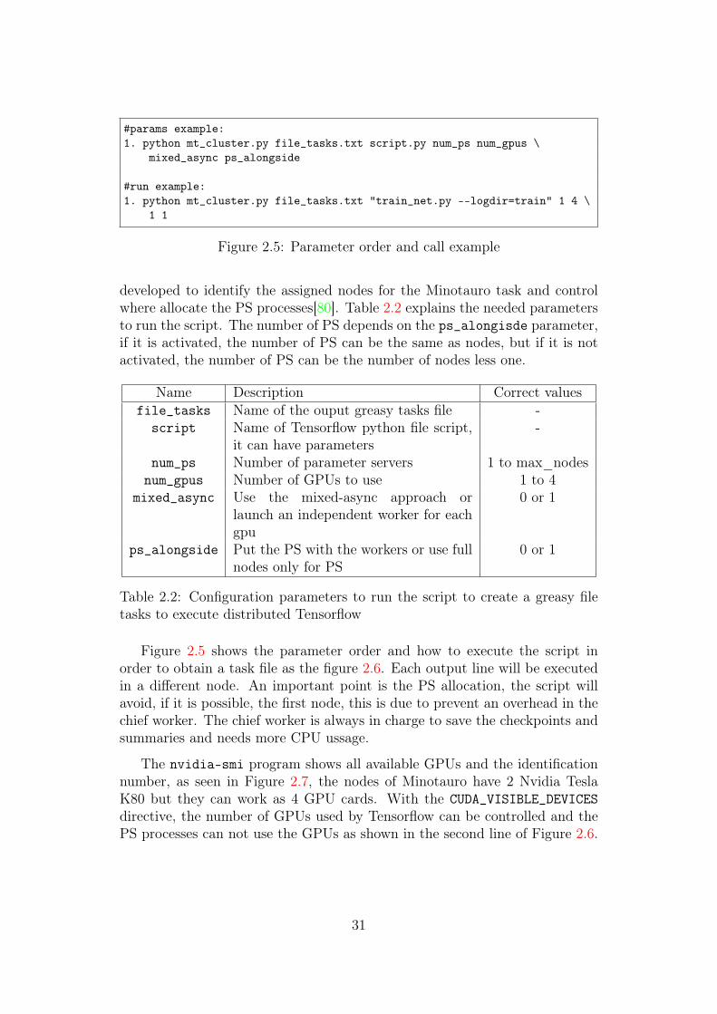
developed to identify the assigned nodes for the Minotauro task and controlwhere allocate the PS processes[80]. Table 2.2 explains the needed parametersto run the script. The number of PS depends on the ps_alongisde parameter,if it is activated, the number of PS can be the same as nodes, but if it is notactivated, the number of PS can be the number of nodes less one.

Name Description Correct valuesfile_tasks Name of the ouput greasy tasks file -

script Name of Tensorflow python file script,it can have parameters

-

num_ps Number of parameter servers 1 to max_nodesnum_gpus Number of GPUs to use 1 to 4

mixed_async Use the mixed-async approach orlaunch an independent worker for eachgpu

0 or 1

ps_alongside Put the PS with the workers or use fullnodes only for PS

0 or 1

Table 2.2: Configuration parameters to run the script to create a greasy filetasks to execute distributed Tensorflow

Figure 2.5 shows the parameter order and how to execute the script inorder to obtain a task file as the figure 2.6. Each output line will be executedin a different node. An important point is the PS allocation, the script willavoid, if it is possible, the first node, this is due to prevent an overhead in thechief worker. The chief worker is always in charge to save the checkpoints andsummaries and needs more CPU ussage.

The nvidia-smi program shows all available GPUs and the identificationnumber, as seen in Figure 2.7, the nodes of Minotauro have 2 Nvidia TeslaK80 but they can work as 4 GPU cards. With the CUDA_VISIBLE_DEVICESdirective, the number of GPUs used by Tensorflow can be controlled and thePS processes can not use the GPUs as shown in the second line of Figure 2.6.

31

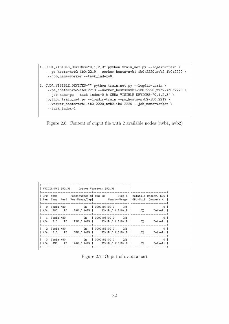
1. CUDA_VISIBLE_DEVICES="0,1,2,3" python train_net.py --logdir=train \--ps_hosts=nvb2-ib0:2219 --worker_hosts=nvb1-ib0:2220,nvb2-ib0:2220 \--job_name=worker --task_index=0

2. CUDA_VISIBLE_DEVICES="" python train_net.py --logdir=train \--ps_hosts=nvb2-ib0:2219 --worker_hosts=nvb1-ib0:2220,nvb2-ib0:2220 \--job_name=ps --task_index=0 & CUDA_VISIBLE_DEVICES="0,1,2,3" \python train_net.py --logdir=train --ps_hosts=nvb2-ib0:2219 \--worker_hosts=nvb1-ib0:2220,nvb2-ib0:2220 --job_name=worker \--task_index=1

Figure 2.6: Content of ouput file with 2 available nodes (nvb1, nvb2)

+------------------------------------------------------+| NVIDIA-SMI 352.39 Driver Version: 352.39 ||-------------------------------+----------------------+----------------------+| GPU Name Persistence-M| Bus-Id Disp.A | Volatile Uncorr. ECC || Fan Temp Perf Pwr:Usage/Cap| Memory-Usage | GPU-Util Compute M. ||===============================+======================+======================|| 0 Tesla K80 On | 0000:04:00.0 Off | 0 || N/A 38C P0 59W / 149W | 22MiB / 11519MiB | 0% Default |+-------------------------------+----------------------+----------------------+| 1 Tesla K80 On | 0000:05:00.0 Off | 0 || N/A 31C P0 72W / 149W | 22MiB / 11519MiB | 0% Default |+-------------------------------+----------------------+----------------------+| 2 Tesla K80 On | 0000:85:00.0 Off | 0 || N/A 31C P0 58W / 149W | 22MiB / 11519MiB | 0% Default |+-------------------------------+----------------------+----------------------+| 3 Tesla K80 On | 0000:86:00.0 Off | 0 || N/A 43C P0 74W / 149W | 22MiB / 11519MiB | 0% Default |+-------------------------------+----------------------+----------------------+

Figure 2.7: Ouput of nvidia-smi

32

2.4.3 Distributed run with Greasy

Greasy is a tool designed to make easier the deployment of embarrassinglyparallel simulations in any environment. It is able to run in parallel a list ofdifferent tasks, schedule them and run them using the available resources.

In order to run Greasy, it is mandatory to load the modules needed by theGreasy tasks and finally, run Greasy passing the task file as parameter:

module load K80 cuda/8.0 mkl/2017.1 CUDNN/5.1.10-cuda_8.0 intel-opencl/2016 python/3.6.0+_ML/apps/GREASY/latest/bin/greasy file_task.txt

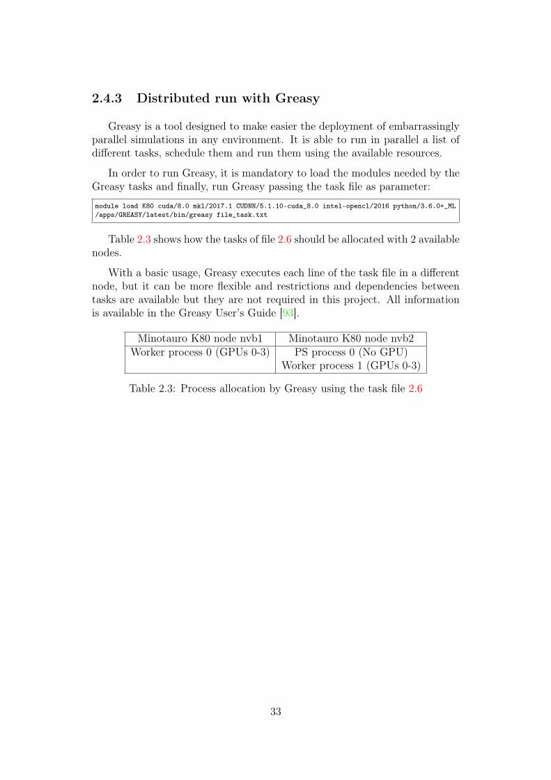
Table 2.3 shows how the tasks of file 2.6 should be allocated with 2 availablenodes.

With a basic usage, Greasy executes each line of the task file in a differentnode, but it can be more flexible and restrictions and dependencies betweentasks are available but they are not required in this project. All informationis available in the Greasy User’s Guide [93].

Minotauro K80 node nvb1 Minotauro K80 node nvb2Worker process 0 (GPUs 0-3) PS process 0 (No GPU)

Worker process 1 (GPUs 0-3)

Table 2.3: Process allocation by Greasy using the task file 2.6

33

34

3. Results

3.1 Throughput and resource usage

3.1.1 Parameter server number

Available publications on distributed training with TensorFlow [2, 20] tendto use different server configurations for worker and parameter server (PS)tasks. Given the PS only stores and updates the model and there is no needfor GPU computations, only CPU servers are used for this task. On the otherhand, most of the worker job involves matrix computations, for which serversequipped with GPUs are used. The Minotauro configuration imposes someconstraints, as the system only has GPU equipped nodes, which means thatplacing PS and workers in different nodes will result in under-utilization ofGPU resources. We decided to study the impact of placing the PS in thesame nodes as the workers, and restricting the resource usage in each task.Odd values of PS are used, because variables are sharded using a round-robinstrategy. Since the weights of the layers take much of the model size, and layerweights and bias are initialized consecutively, we want to have them as muchdistributed as possible, hence the use of an odd value.

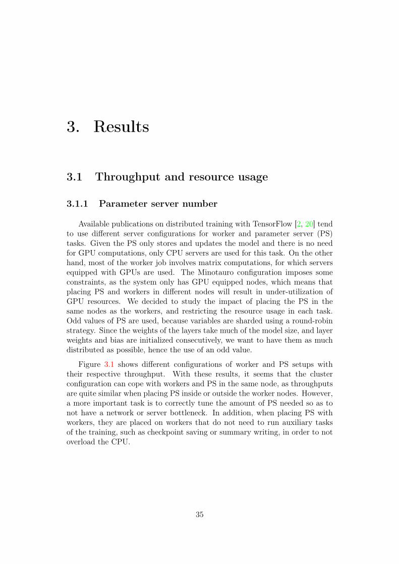
Figure 3.1 shows different configurations of worker and PS setups withtheir respective throughput. With these results, it seems that the clusterconfiguration can cope with workers and PS in the same node, as throughputsare quite similar when placing PS inside or outside the worker nodes. However,a more important task is to correctly tune the amount of PS needed so as tonot have a network or server bottleneck. In addition, when placing PS withworkers, they are placed on workers that do not need to run auxiliary tasksof the training, such as checkpoint saving or summary writing, in order to notoverload the CPU.

35

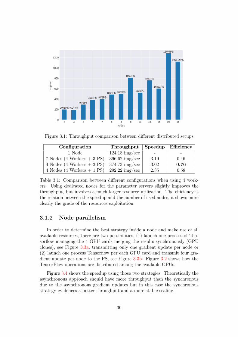
Figure 3.1: Throughput comparison between different distributed setups

Configuration Throughput Speedup Efficiency1 Node 124.18 img/sec - -

7 Nodes (4 Workers + 3 PS) 396.62 img/sec 3.19 0.464 Nodes (4 Workers + 3 PS) 374.73 img/sec 3.02 0.764 Nodes (4 Workers + 1 PS) 292.22 img/sec 2.35 0.58

Table 3.1: Comparison between different configurations when using 4 work-ers. Using dedicated nodes for the parameter servers slightly improves thethroughput, but involves a much larger resource utilization. The efficiency isthe relation between the speedup and the number of used nodes, it shows moreclearly the grade of the resources exploitation.

3.1.2 Node parallelism

In order to determine the best strategy inside a node and make use of allavailable resources, there are two possibilities, (1) launch one process of Ten-sorflow managing the 4 GPU cards merging the results synchronously (GPUclones), see Figure 3.3a, transmitting only one gradient update per node or(2) launch one process Tensorflow per each GPU card and transmit four gra-dient update per node to the PS, see Figure 3.3b. Figure 3.2 shows how theTensorFlow operations are distributed among the available GPUs.

Figure 3.4 shows the speedup using those two strategies. Theoretically theasynchronous approach should have more throughput than the synchronousdue to the asynchronous gradient updates but in this case the synchronousstrategy evidences a better throughput and a more stable scaling.

36

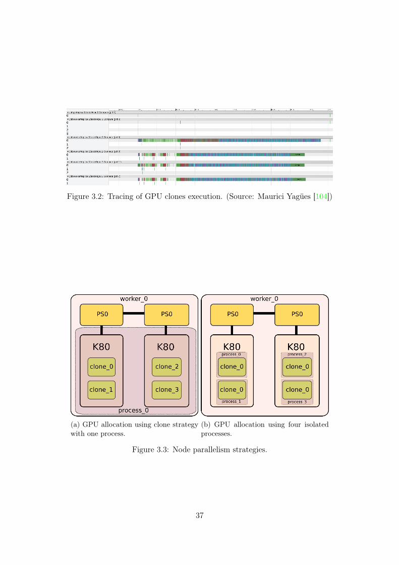
Figure 3.2: Tracing of GPU clones execution. (Source: Maurici Yagües [104])

(a) GPU allocation using clone strategywith one process.

(b) GPU allocation using four isolatedprocesses.

Figure 3.3: Node parallelism strategies.

37

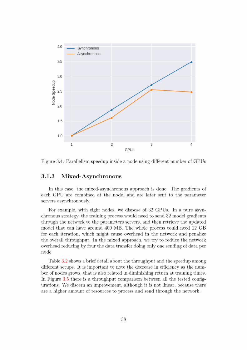
Figure 3.4: Parallelism speedup inside a node using different number of GPUs

3.1.3 Mixed-Asynchronous

In this case, the mixed-asynchronous approach is done. The gradients ofeach GPU are combined at the node, and are later sent to the parameterservers asynchronously.

For example, with eight nodes, we dispose of 32 GPUs. In a pure asyn-chronous strategy, the training process would need to send 32 model gradientsthrough the network to the parameters servers, and then retrieve the updatedmodel that can have around 400 MB. The whole process could need 12 GBfor each iteration, which might cause overhead in the network and penalizethe overall throughput. In the mixed approach, we try to reduce the networkoverhead reducing by four the data transfer doing only one sending of data pernode.

Table 3.2 shows a brief detail about the throughput and the speedup amongdifferent setups. It is important to note the decrease in efficiency as the num-ber of nodes grows, that is also related in diminishing return at training times.In Figure 3.5 there is a throughput comparison between all the tested config-urations. We discern an improvement, although it is not linear, because thereare a higher amount of resources to process and send through the network.

38

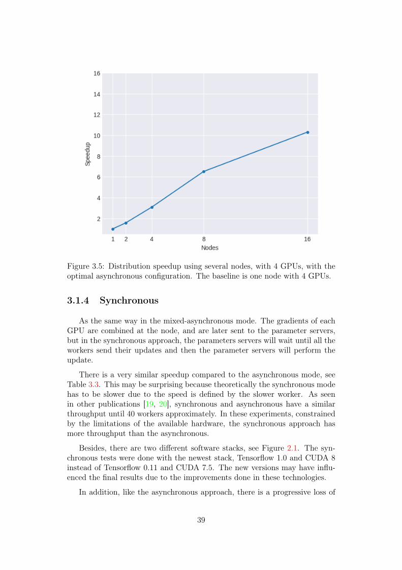
Figure 3.5: Distribution speedup using several nodes, with 4 GPUs, with theoptimal asynchronous configuration. The baseline is one node with 4 GPUs.

3.1.4 Synchronous

As the same way in the mixed-asynchronous mode. The gradients of eachGPU are combined at the node, and are later sent to the parameter servers,but in the synchronous approach, the parameters servers will wait until all theworkers send their updates and then the parameter servers will perform theupdate.

There is a very similar speedup compared to the asynchronous mode, seeTable 3.3. This may be surprising because theoretically the synchronous modehas to be slower due to the speed is defined by the slower worker. As seenin other publications [19, 20], synchronous and asynchronous have a similarthroughput until 40 workers approximately. In these experiments, constrainedby the limitations of the available hardware, the synchronous approach hasmore throughput than the asynchronous.

Besides, there are two different software stacks, see Figure 2.1. The syn-chronous tests were done with the newest stack, Tensorflow 1.0 and CUDA 8instead of Tensorflow 0.11 and CUDA 7.5. The new versions may have influ-enced the final results due to the improvements done in these technologies.

In addition, like the asynchronous approach, there is a progressive loss of

39

Setup Throughput Speedup Efficiency1 Node (No distribution) 124.18 img/sec - -

2 Nodes (2 Workers + 1 PS) 195.60 img/sec 1.58 0.794 Nodes (4 Workers + 3 PS) 383.09 img/sec 3.09 0.778 Nodes (8 Workers + 7 PS) 809.10 img/sec 6.52 0.8216 Nodes (16 Workers + 7 PS) 1278.53 img/sec 10.30 0.64

Table 3.2: Speedup comparing a single node between different asynchronousdistributed configurations and their speedup-resources relation.

Setup Throughput Speedup Efficiency1 Node (No distribution) 124.18 img/sec - -

2 Nodes (2 Workers + 1 PS) 216.32 img/sec 1.74 0.874 Nodes (4 Workers + 3 PS) 401.09 img/sec 3.23 0.808 Nodes (8 Workers + 7 PS) 758.64 img/sec 6.11 0.7616 Nodes (16 Workers + 7 PS) 1311.37 img/sec 10.56 0.66

Table 3.3: Speedup comparing a single node between different synchronousdistributed configurations and their speedup-resources relation.

throughput. The more nodes, the more loss but in this case, the synchronousachieves better efficiency and speedup results than mixed-asynchronous.

3.2 Learning time

When studying the impact of distribution on the training process, there aretwo main factors to take into account. First, the time required for the modelto reach a target loss value, which is the target function being optimized,determines which is the speedup on the training process. Second, the finalaccuracy determines how the asynchronous/syncrhonous updates affect theoptimization of the cost function.

3.2.1 Mixed-Asynchronous

Despite the throughput increase is close to linear with respect to the numberof nodes, Figure 3.7 shows how the time required by each setup to reach a targetloss value does not benefit linearly from the additional nodes. This result isexpected, since for an asynchronous gradient descent method with N workerseach model update is performed with respect to weights wich are N − 1 stepsold on average.

The final accuracies on the test set reached by each configuration are de-

40

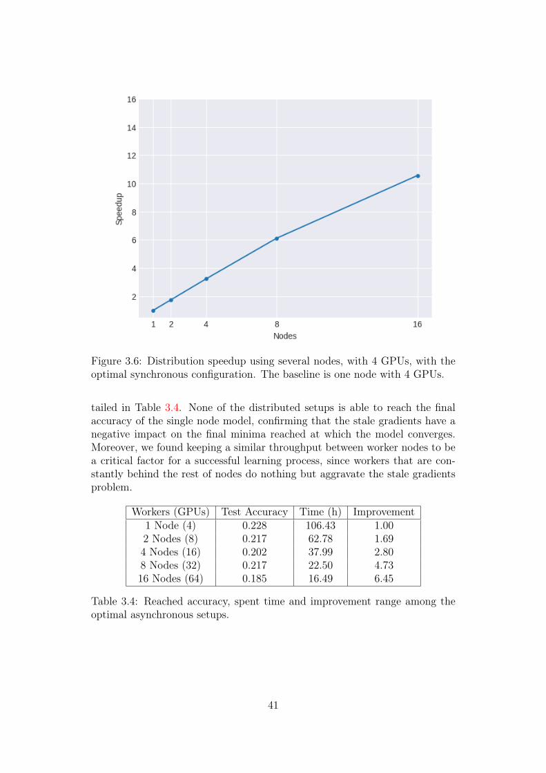
Figure 3.6: Distribution speedup using several nodes, with 4 GPUs, with theoptimal synchronous configuration. The baseline is one node with 4 GPUs.

tailed in Table 3.4. None of the distributed setups is able to reach the finalaccuracy of the single node model, confirming that the stale gradients have anegative impact on the final minima reached at which the model converges.Moreover, we found keeping a similar throughput between worker nodes to bea critical factor for a successful learning process, since workers that are con-stantly behind the rest of nodes do nothing but aggravate the stale gradientsproblem.

Workers (GPUs) Test Accuracy Time (h) Improvement1 Node (4) 0.228 106.43 1.002 Nodes (8) 0.217 62.78 1.694 Nodes (16) 0.202 37.99 2.808 Nodes (32) 0.217 22.50 4.7316 Nodes (64) 0.185 16.49 6.45

Table 3.4: Reached accuracy, spent time and improvement range among theoptimal asynchronous setups.

41

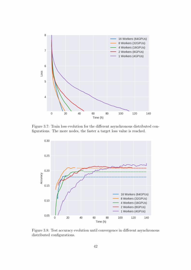
Figure 3.7: Train loss evolution for the different asynchronous distributed con-figurations. The more nodes, the faster a target loss value is reached.

Figure 3.8: Test accuracy evolution until convergence in different asynchronousdistributed configurations.

42

3.2.2 Synchronous

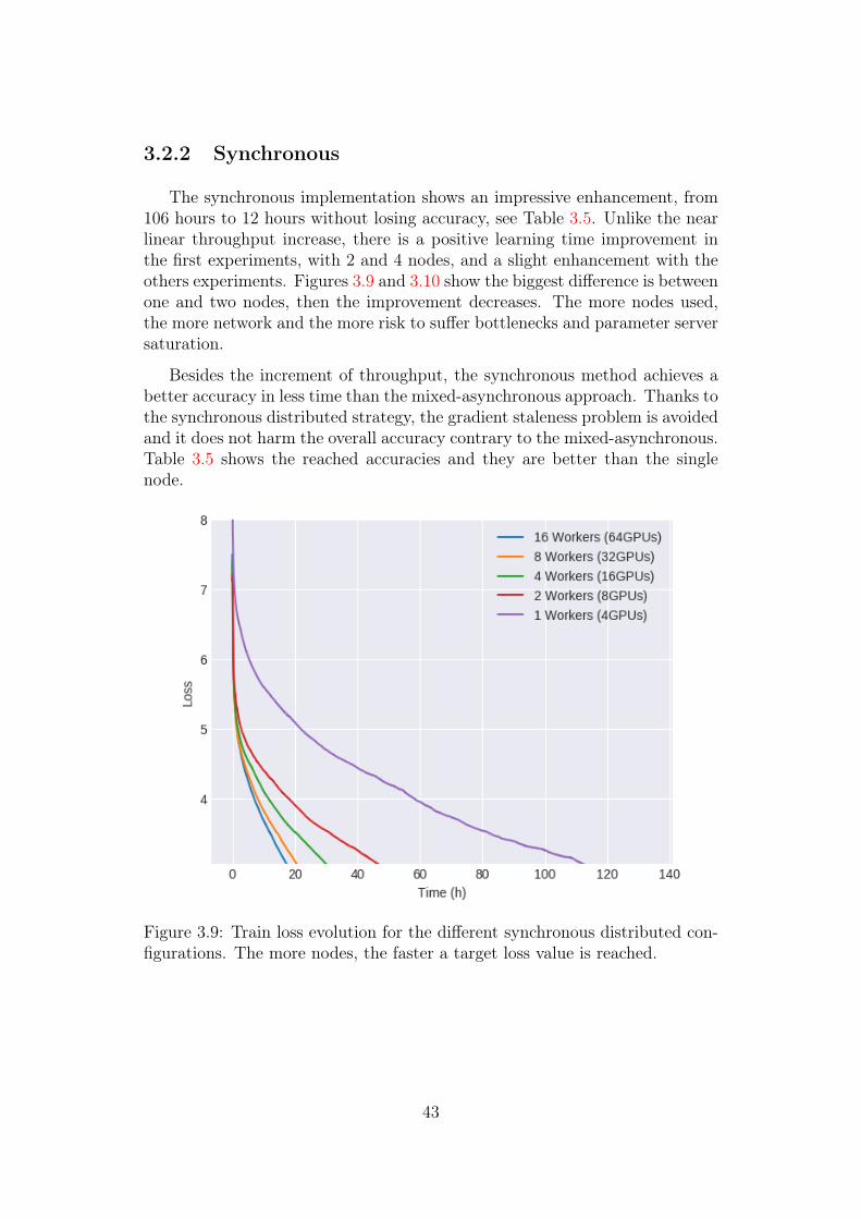
The synchronous implementation shows an impressive enhancement, from106 hours to 12 hours without losing accuracy, see Table 3.5. Unlike the nearlinear throughput increase, there is a positive learning time improvement inthe first experiments, with 2 and 4 nodes, and a slight enhancement with theothers experiments. Figures 3.9 and 3.10 show the biggest difference is betweenone and two nodes, then the improvement decreases. The more nodes used,the more network and the more risk to suffer bottlenecks and parameter serversaturation.

Besides the increment of throughput, the synchronous method achieves abetter accuracy in less time than the mixed-asynchronous approach. Thanks tothe synchronous distributed strategy, the gradient staleness problem is avoidedand it does not harm the overall accuracy contrary to the mixed-asynchronous.Table 3.5 shows the reached accuracies and they are better than the singlenode.

Figure 3.9: Train loss evolution for the different synchronous distributed con-figurations. The more nodes, the faster a target loss value is reached.

43

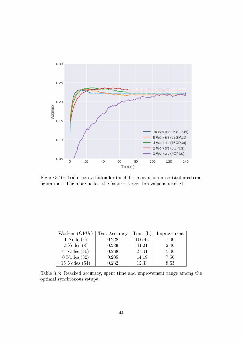
Figure 3.10: Train loss evolution for the different synchronous distributed con-figurations. The more nodes, the faster a target loss value is reached.

Workers (GPUs) Test Accuracy Time (h) Improvement1 Node (4) 0.228 106.43 1.002 Nodes (8) 0.239 44.21 2.404 Nodes (16) 0.238 21.01 5.068 Nodes (32) 0.235 14.19 7.5016 Nodes (64) 0.232 12.33 8.63

Table 3.5: Reached accuracy, spent time and improvement range among theoptimal synchronous setups.

44

3.2.3 Comparing strategies

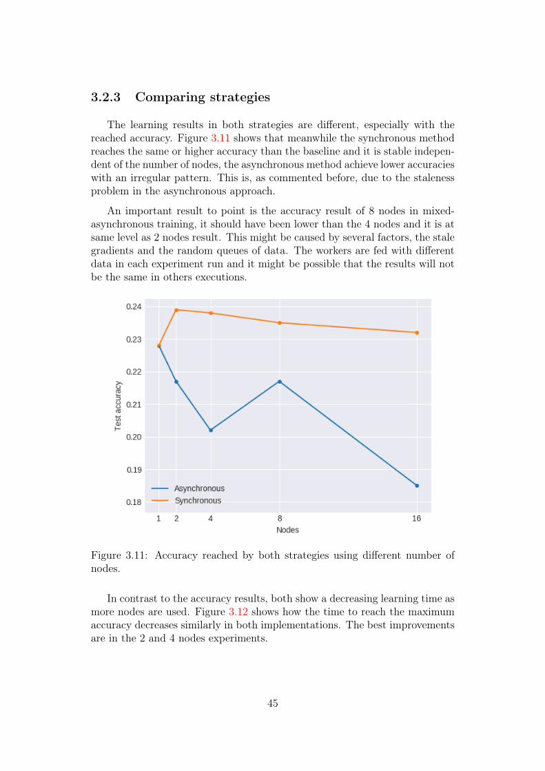
The learning results in both strategies are different, especially with thereached accuracy. Figure 3.11 shows that meanwhile the synchronous methodreaches the same or higher accuracy than the baseline and it is stable indepen-dent of the number of nodes, the asynchronous method achieve lower accuracieswith an irregular pattern. This is, as commented before, due to the stalenessproblem in the asynchronous approach.

An important result to point is the accuracy result of 8 nodes in mixed-asynchronous training, it should have been lower than the 4 nodes and it is atsame level as 2 nodes result. This might be caused by several factors, the stalegradients and the random queues of data. The workers are fed with differentdata in each experiment run and it might be possible that the results will notbe the same in others executions.

Figure 3.11: Accuracy reached by both strategies using different number ofnodes.

In contrast to the accuracy results, both show a decreasing learning time asmore nodes are used. Figure 3.12 shows how the time to reach the maximumaccuracy decreases similarly in both implementations. The best improvementsare in the 2 and 4 nodes experiments.

45

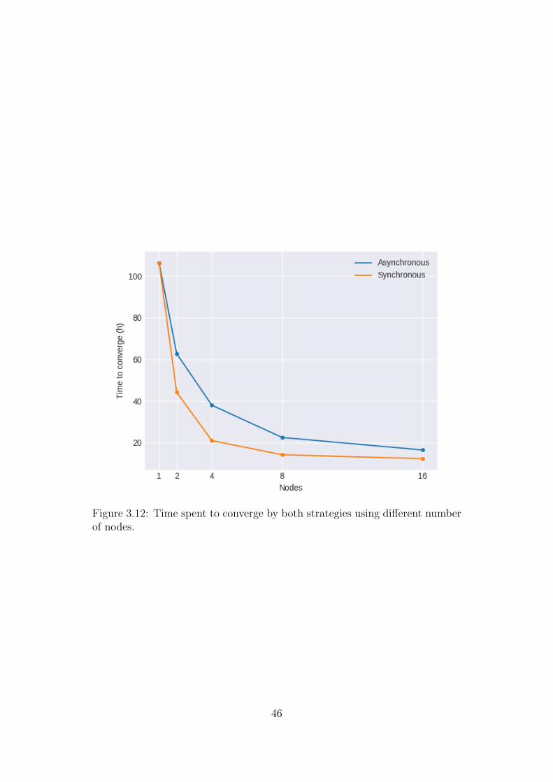
Figure 3.12: Time spent to converge by both strategies using different numberof nodes.

46

4. Conclusions

Next years, Deep Learning will become more important everyday. TheDeep Learning processes will have to be done in the shortest possible time,besides the amount of data to be processed does not stop increasing everyday.This boost of requirements will allow Deep Learning to encompass more fieldsand face more complex achievements. High performance computers have tohelp Deep Learning to go further and to do it faster.

4.1 Project outcomes

Barcelona Supercomputing Center strategic vision

This work shows that Deep Learning can be accelerated using high perfor-mance computers and applied in ones that were not created for this purpose.With these results, Barcelona Supercomputing Center may change its strategicvision about Deep Learning and may start new research fields. Besides, thiswork explains how to deploy a Deep Learning cluster inside its infrastructures.

Resource usage optimization

In this project, different modes to optimize the available resources havebeen evaluated. First, we observed that placing the parameter servers in thesame machine as the worker processes does not affect in a significant waycompared to the poor improvement putting the same parameters servers alonein others machines. Additionally, we checked different approaches for usingall the GPUs in a node, launching a different process per GPU or using onlyone process an merge the results from each GPU before sending them to theparameter servers.

47

Results and costs

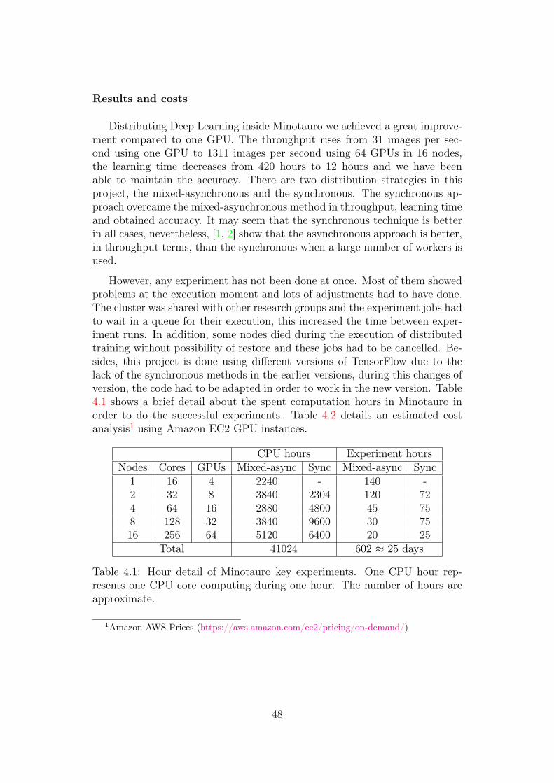
Distributing Deep Learning inside Minotauro we achieved a great improve-ment compared to one GPU. The throughput rises from 31 images per sec-ond using one GPU to 1311 images per second using 64 GPUs in 16 nodes,the learning time decreases from 420 hours to 12 hours and we have beenable to maintain the accuracy. There are two distribution strategies in thisproject, the mixed-asynchronous and the synchronous. The synchronous ap-proach overcame the mixed-asynchronous method in throughput, learning timeand obtained accuracy. It may seem that the synchronous technique is betterin all cases, nevertheless, [1, 2] show that the asynchronous approach is better,in throughput terms, than the synchronous when a large number of workers isused.

However, any experiment has not been done at once. Most of them showedproblems at the execution moment and lots of adjustments had to have done.The cluster was shared with other research groups and the experiment jobs hadto wait in a queue for their execution, this increased the time between exper-iment runs. In addition, some nodes died during the execution of distributedtraining without possibility of restore and these jobs had to be cancelled. Be-sides, this project is done using different versions of TensorFlow due to thelack of the synchronous methods in the earlier versions, during this changes ofversion, the code had to be adapted in order to work in the new version. Table4.1 shows a brief detail about the spent computation hours in Minotauro inorder to do the successful experiments. Table 4.2 details an estimated costanalysis1 using Amazon EC2 GPU instances.

CPU hours Experiment hoursNodes Cores GPUs Mixed-async Sync Mixed-async Sync

1 16 4 2240 - 140 -2 32 8 3840 2304 120 724 64 16 2880 4800 45 758 128 32 3840 9600 30 7516 256 64 5120 6400 20 25

Total 41024 602 ≈ 25 days

Table 4.1: Hour detail of Minotauro key experiments. One CPU hour rep-resents one CPU core computing during one hour. The number of hours areapproximate.

1Amazon AWS Prices (https://aws.amazon.com/ec2/pricing/on-demand/)

48

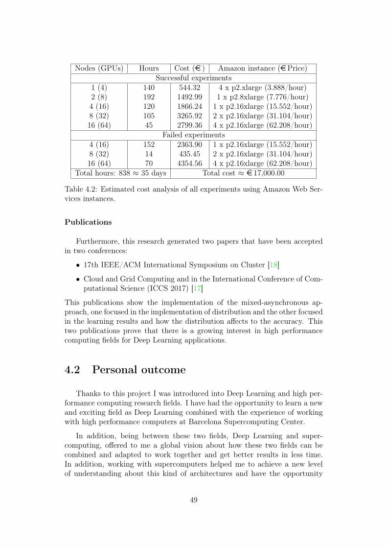
Nodes (GPUs) Hours Cost (e ) Amazon instance (ePrice)Successful experiments

1 (4) 140 544.32 4 x p2.xlarge (3.888/hour)2 (8) 192 1492.99 1 x p2.8xlarge (7.776/hour)4 (16) 120 1866.24 1 x p2.16xlarge (15.552/hour)8 (32) 105 3265.92 2 x p2.16xlarge (31.104/hour)16 (64) 45 2799.36 4 x p2.16xlarge (62.208/hour)

Failed experiments4 (16) 152 2363.90 1 x p2.16xlarge (15.552/hour)8 (32) 14 435.45 2 x p2.16xlarge (31.104/hour)16 (64) 70 4354.56 4 x p2.16xlarge (62.208/hour)

Total hours: 838 ≈ 35 days Total cost ≈ e 17,000.00

Table 4.2: Estimated cost analysis of all experiments using Amazon Web Ser-vices instances.

Publications

Furthermore, this research generated two papers that have been acceptedin two conferences:

• 17th IEEE/ACM International Symposium on Cluster [18]

• Cloud and Grid Computing and in the International Conference of Com-putational Science (ICCS 2017) [17]

This publications show the implementation of the mixed-asynchronous ap-proach, one focused in the implementation of distribution and the other focusedin the learning results and how the distribution affects to the accuracy. Thistwo publications prove that there is a growing interest in high performancecomputing fields for Deep Learning applications.

4.2 Personal outcome

Thanks to this project I was introduced into Deep Learning and high per-formance computing research fields. I have had the opportunity to learn a newand exciting field as Deep Learning combined with the experience of workingwith high performance computers at Barcelona Supercomputing Center.

In addition, being between these two fields, Deep Learning and super-computing, offered to me a global vision about how these two fields can becombined and adapted to work together and get better results in less time.In addition, working with supercomputers helped me to achieve a new levelof understanding about this kind of architectures and have the opportunity

49

of using technologies such CUDA or MPI that I could not use in traditionalenvironments. On the other hand, acquiring knowledge about Deep Learninghas been very valuable in order to increase my background and be able toapply this expertise in the future.

To finish, during this project I faced different difficulties. Starting with anew framework such TensorFlow is not easy, it has a high learning curve dueto the graph paradigm that it follows. Another point was the Deep Learningworld, I was familiar with some DL concepts but they were just the tip of theiceberg, I had to immerse in a exciting but complex universe. On the otherhand I have learned that working with big computers entails bigger problemsand more convoluted solutions.

4.3 Future work

This job may embrace several research areas. Firstly, we would test thissolution in bigger heterogeneous machines with more nodes and different struc-tures in order to test if this solution is scalable in bigger environments and provewhich strategy is better for different clusters. The MareNostrum 4 supercom-puter will offer new Intel Knights Landing and IBM POWER9 processors withnew Nvidia GPUs clusters2, with these new technologies available for research,it would be intriguing to try this solution on these new clusters. Besides, aproper implementation of TensorFlow using PyCOMPSs [94] instead gRPCand the Tensorflow distributed routines may be valubale for showing if Py-COMPSs implementation might be an alternative for the BSC infrastructuresinstead of the generic implementation of TensorFlow. Also, TensorFlow willsupport RDMA3 in a near future and comparing the results of this thesis withones using RDMA will be intriguing. In addition, compare these results withthe results from other frameworks such as Caffe2 or PyTorch may be valuable.

Owing to the lack of nodes, there is another strategy that we could not test,the synchronous gradient descent with backup workers. Prove this strategy andcompare it to the asynchronous in larger machines would be interesting.

Nowadays, there are some projects in order to create new tools to managea TensorFlow cluster, one of this tools is TensorFlowOnSpark4, developed bythe Yahoo Hadoop Team, that permits to use Spark5 to manage a cluster ofTensorFlow and combine Spark and Hadoop data sources with TensorFlow.

2BSC press release (https://www.bsc.es/news/bsc-news/marenostrum-4-supercomputer-be-12-times-more-powerful-marenostrum-3)

3A Tutorial of the RDMAModel (https://www.hpcwire.com/2006/09/15/a_tutorial_of_the_rdma_model-1/)

4Yahoo Hadoop Blog (http://yahoohadoop.tumblr.com/post/157196317141/open-sourcing-tensorflowonspark-distributed-deep)

5Apache Spark Website (http://spark.apache.org/)

50

This will be useful for implementing TensorFlow on existing Big Data clustersthat operate with Spark. This kind of initiatives help to expand the domainsof TensorFlow to production environments.

To finish, at the moment there are tools to use TensorFlow as a servicelike Floyd Hub6, this service allows to upload a TensorFlow code and run itwithout caring about the system setup. Nevertheless it does not support dis-tribution and it is constrained to the number of GPUs available on the virtualmachines. Creating a tool for researchers may be valuable, a tool that would al-low researchers to run distributed TensorFlow porcesses without regard aboutnetwork parameters, GPU configurations or parallelism management. Simplysending the code to the tool. A tool of this kind will prevent researchers towaste time dealing with problems about distribution.

6Floyd Hub Website (https://www.floydhub.com/)

51

52

Bibliography

[1] Martın Abadi et al. “TensorFlow: Large-scale machine learning on het-erogeneous systems”. In: (2015).

[2] M. Abadi et al. “TensorFlow: A system for large-scale machine learning”.In: ArXiv e-prints (May 2016). arXiv: 1605.08695 [cs.DC].

[3] Zeynep Akata, Florent Perronnin, Zaid Harchaoui, and Cordelia Schmid.“Label-embedding for image classification”. In: IEEE transactions onpattern analysis and machine intelligence (2016).

[4] Norman P. Jouppi et al. “In-Datacenter Performance Analysis of a Ten-sor Processing Unit”. In: ISCA (2017).

[5] Víctor Campos et al. “Sentiment Concept Embedding for Visual AffectRecognition”. 2017.

[6] Soheil Bahrampour, Naveen Ramakrishnan, Lukas Schott, and MohakShah. “Comparative Study of Caffe, Neon, Theano, and for Deep Learn-ing”. In: CoRR abs/1511.06435 (2015). url: http://arxiv.org/abs/1511.06435.

[7] Marco Baroni and Roberto Zamparelli. “Nouns are vectors, adjectivesare matrices: Representing adjective-noun constructions in semanticspace”. In: EMNLP. 2010.

[8] James Bergstra et al. “Theano: Deep learning on gpus with python”.In: NIPS Workshops. 2011.

[9] Gedas Bertasius, Jianbo Shi, and Lorenzo Torresani. “DeepEdge: AMulti-Scale Bifurcated Deep Network for Top-Down Contour Detec-tion”. In: CoRR abs/1412.1123 (2014). url: http://arxiv.org/abs/1412.1123.

[10] Damian Borth, Tao Chen, Rongrong Ji, and Shih-Fu Chang. “Sen-tibank: large-scale ontology and classifiers for detecting sentiment andemotions in visual content”. In: ACM MM. 2013.

[11] Damian Borth, Rongrong Ji, Tao Chen, Thomas Breuel, and Shih-FuChang. “Large-scale visual sentiment ontology and detectors using ad-jective noun pairs”. In: ACM MM. 2013.

53

[12] Barcelona Supercomputing Center BSC. About BSC. 2016. url: https://www.bsc.es/discover-bsc/the-centre/what-we-do.

[13] Barcelona Supercomputing Center BSC.MinoTauro User’s Guide. 2016.url: http://www.bsc.es/support/MinoTauro-ug.pdf.

[14] Fabian Caba Heilbron, Victor Escorcia, Bernard Ghanem, and JuanCarlos Niebles. “Activitynet: A large-scale video benchmark for hu-man activity understanding”. In: Proceedings of the IEEE Conferenceon Computer Vision and Pattern Recognition. 2015, pp. 961–970.

[15] Michel Cabanac. “What is emotion?” In: Behavioural processes 60.2(2002).

[16] Victor Campos, Amaia Salvador, Brendan Jou, and Xavier Giro-i-Nieto.“Diving Deep into Sentiment: Understanding Fine-tuned CNNs for Vi-sual Sentiment Prediction”. In: ASM, ACM MM Workshops. 2015.

[17] Víctor Campos, Francesc Sastre, Maurici Yagües, Míriam Bellver, XavierGiró-i-Nieto, and Jordi Torres. “Distributed training strategies for acomputer vision deep learning algorithm on a distributed GPU clus-ter”. 2017.

[18] Víctor Campos, Francesc Sastre, Maurici Yagües, Xavier Giró-i-Nieto,and Jordi Torres. “Scaling a Convolutional Neural Network for classi-fication of Adjective Noun Pairs with TensorFlow on GPU Clusters”.2017.

[19] Jianmin Chen, Rajat Monga, Samy Bengio, and Rafal Jozefowicz. “Re-visiting Distributed Synchronous SGD”. In: ICLR Workshops. 2016.

[20] Jianmin Chen, Xinghao Pan, Rajat Monga, Samy Bengio, and RafalJozefowicz. “Revisiting Distributed Synchronous SGD”. ICLR 2017 con-ference submission. 2016.

[21] Tao Chen, Damian Borth, Trevor Darrell, and Shih-Fu Chang. “DeepSen-tiBank: Visual sentiment concept classification with deep convolutionalneural networks”. In: arXiv:1410.8586 (2014).

[22] Tianqi Chen et al. “Mxnet: A flexible and efficient machine learn-ing library for heterogeneous distributed systems”. In: arXiv preprintarXiv:1512.01274 (2015).

[23] Sharan Chetlur, Cliff Woolley, Philippe Vandermersch, Jonathan Co-hen, John Tran, Bryan Catanzaro, and Evan Shelhamer. “cudnn: Effi-cient primitives for deep learning”. In: arXiv preprint arXiv:1410.0759(2014).

54

[24] Adam Coates, Brody Huval, Tao Wang, David Wu, Bryan catanzaro,and Ng Andrew. “Deep learning with COTS HPC systems”. In: Proceed-ings of the 30th International Conference on Machine learning (ICML-13). Ed. by Sanjoy Dasgupta and David Mcallester. Vol. 28. 3. JMLRWorkshop and Conference Proceedings, 2013, pp. 1337–1345. url: http://jmlr.org/proceedings/papers/v28/coates13.pdf.

[25] Ronan Collobert, Koray Kavukcuoglu, and Clément Farabet. “7: AMatlab-like Environment for Machine Learning”. In: BigLearn, NIPSWorkshop. 2011.

[26] Michael Copeland. The Difference Between AI, Machine Learning, andDeep Learning? | NVIDIA Blog. 2016. url: https://blogs.nvidia.com/blog/2016/07/29/whats-difference-artificial-intelligence-machine-learning-deep-learning-ai/ (visited on 04/25/2017).

[27] Henggang Cui, Hao Zhang, Gregory R. Ganger, Phillip B. Gibbons,and Eric P. Xing. “GeePS: Scalable Deep Learning on Distributed GPUswith a GPU-specialized Parameter Server”. In: Proceedings of the EleventhEuropean Conference on Computer Systems. EuroSys ’16. London, UnitedKingdom: ACM, 2016, 4:1–4:16. doi: 10.1145/2901318.2901323.

[28] Jifeng Dai, Yi Li, Kaiming He, and Jian Sun. “R-FCN: Object Detectionvia Region-based Fully Convolutional Networks”. In: CoRR abs/1605.06409(2016). url: http://arxiv.org/abs/1605.06409.

[29] Zhenwen Dai, Andreas C. Damianou, Javier González, and Neil D.Lawrence. “Variational Auto-encoded Deep Gaussian Processes”. In:CoRR abs/1511.06455 (2015). url: http://arxiv.org/abs/1511.06455.

[30] Vaidehi Dalmia, Hongyi Liu, and Shih-Fu Chang. “Columbia MVSOImage Sentiment Dataset”. In: arXiv preprint arXiv:1611.04455 (2016).

[31] Jia Deng, Wei Dong, Richard Socher, Li-Jia Li, Kai Li, and Li Fei-Fei.“ImageNet: A large-scale hierarchical image database”. In: CVPR. 2009.

[32] Chao Dong, Yubin Deng, Chen Change Loy, and Xiaoou Tang. “Com-pression Artifacts Reduction by a Deep Convolutional Network”. In:CoRR abs/1504.06993 (2015). url: http://arxiv.org/abs/1504.06993.

[33] Chao Dong, Chen Change Loy, Kaiming He, and Xiaoou Tang. “Im-age Super-Resolution Using Deep Convolutional Networks”. In: CoRRabs/1501.00092 (2015). url: http://arxiv.org/abs/1501.00092.

[34] Andrea Frome, Greg S Corrado, Jon Shlens, Samy Bengio, Jeff Dean,Tomas Mikolov, et al. “Devise: A deep visual-semantic embedding model”.In: NIPS. 2013.

[35] Ross B. Girshick. “Fast R-CNN”. In: CoRR abs/1504.08083 (2015). url:http://arxiv.org/abs/1504.08083.

55

[36] Ross B. Girshick, Jeff Donahue, Trevor Darrell, and Jitendra Malik.“Rich feature hierarchies for accurate object detection and semanticsegmentation”. In: CoRR abs/1311.2524 (2013). url: http://arxiv.org/abs/1311.2524.

[37] I. J. Goodfellow, J. Pouget-Abadie, M. Mirza, B. Xu, D. Warde-Farley,S. Ozair, A. Courville, and Y. Bengio. “Generative Adversarial Net-works”. In: ArXiv e-prints (June 2014). arXiv: 1406.2661 [stat.ML].

[38] Kaiming He, Xiangyu Zhang, Shaoqing Ren, and Jian Sun. “Deep Resid-ual Learning for Image Recognition”. In: CVPR. 2016.

[39] Eduard H Hovy. “What are Sentiment, Affect, and Emotion? Applyingthe Methodology of Michael Zock to Sentiment Analysis”. In: LanguageProduction, Cognition, and the Lexicon 48 (2014).

[40] Jonathan Huang et al. “Speed/accuracy trade-offs for modern convolu-tional object detectors”. In: CoRR abs/1611.10012 (2016). url: http://arxiv.org/abs/1611.10012.

[41] Yangqing Jia, Evan Shelhamer, Jeff Donahue, Sergey Karayev, JonathanLong, Ross Girshick, Sergio Guadarrama, and Trevor Darrell. “Caffe:Convolutional architecture for fast feature embedding”. In: ACM MM.2014.

[42] Yu-Gang Jiang, Baohan Xu, and Xiangyang Xue. “Predicting Emotionsin User-Generated Videos.” In: AAAI. 2014.

[43] Peter H Jin, Qiaochu Yuan, Forrest Iandola, and Kurt Keutzer. “How toscale distributed deep learning?” In: arXiv preprint arXiv:1611.04581(2016).

[44] Brendan Jou and Shih-Fu Chang. “Deep Cross Residual Learning forMultitask Visual Recognition”. In: ACM MM. 2016.

[45] Brendan Jou and Shih-Fu Chang. “Going Deeper for Multilingual VisualSentiment Detection”. In: arXiv preprint arXiv:1605.09211 (2016).

[46] Brendan Jou, Tao Chen, Nikolaos Pappas, Miriam Redi, Mercan Top-kara, and Shih-Fu Chang. “Visual affect around the world: A large-scalemultilingual visual sentiment ontology”. In: ACM MM. 2015.

[47] Andrej Karpathy and Fei-Fei Li. “Deep Visual-Semantic Alignments forGenerating Image Descriptions”. In: CoRR abs/1412.2306 (2014). url:http://arxiv.org/abs/1412.2306.

[48] Andrej Karpathy, George Toderici, Sanketh Shetty, Thomas Leung,Rahul Sukthankar, and Li Fei-Fei. “Large-scale video classification withconvolutional neural networks”. In: CVPR. 2014.

[49] Nitish Shirish Keskar, Dheevatsa Mudigere, Jorge Nocedal, MikhailSmelyanskiy, and Ping Tak Peter Tang. “On large-batch training fordeep learning: Generalization gap and sharp minima”. In: arXiv preprintarXiv:1609.04836 (2016).

56

[50] Alex Krizhevsky. “One weird trick for parallelizing convolutional neuralnetworks”. In: arXiv preprint arXiv:1404.5997 (2014).

[51] Alex Krizhevsky, Ilya Sutskever, and Geoffrey E. Hinton. “ImageNetClassification with Deep Convolutional Neural Networks”. In: NIPS.2012.

[52] Richard D Lane and Lynn Nadel. Cognitive neuroscience of emotion.Oxford University Press, USA, 2002.

[53] Yann LeCun, Yoshua Bengio, and Geoffrey Hinton. “Deep learning”. In:Nature 521.7553 (May 2015), pp. 436–444. doi: 10.1038/nature14539.

[54] Yann LeCun, Léon Bottou, Yoshua Bengio, and Patrick Haffner. “Gradient-based learning applied to document recognition”. In: Proceedings of theIEEE 86.11 (1998).

[55] Christian Ledig, Lucas Theis, Ferenc Huszar, Jose Caballero, AndrewP. Aitken, Alykhan Tejani, Johannes Totz, Zehan Wang, and WenzheShi. “Photo-Realistic Single Image Super-Resolution Using a GenerativeAdversarial Network”. In: CoRR abs/1609.04802 (2016). url: http://arxiv.org/abs/1609.04802.

[56] Wei Liu, Dragomir Anguelov, Dumitru Erhan, Christian Szegedy, ScottE. Reed, Cheng-Yang Fu, and Alexander C. Berg. “SSD: Single ShotMultiBox Detector”. In: CoRR abs/1512.02325 (2015). url: http://arxiv.org/abs/1512.02325.

[57] He Ma, Fei Mao, and GrahamW Taylor. “Theano-MPI: a Theano-basedDistributed Training Framework”. In: arXiv preprint arXiv:1605.08325(2016).

[58] Jana Machajdik and Allan Hanbury. “Affective Image ClassificationUsing Features Inspired by Psychology and Art Theory”. In: ACM MM.2010.

[59] Junhua Mao, Wei Xu, Yi Yang, Jiang Wang, and Alan L. Yuille. “Ex-plain Images with Multimodal Recurrent Neural Networks”. In: CoRRabs/1410.1090 (2014). url: http://arxiv.org/abs/1410.1090.

[60] Daniel McDuff, Rana El Kaliouby, Jeffrey F Cohn, and Rosalind W Pi-card. “Predicting ad liking and purchase intent: Large-scale analysis offacial responses to ads”. In: IEEE Transactions on Affective Computing6.3 (2015).

[61] Tomas Mikolov, Kai Chen, Greg Corrado, and Jeffrey Dean. “Efficientestimation of word representations in vector space”. In: ICLR. 2013.

[62] Tomas Mikolov, Ilya Sutskever, Kai Chen, Greg S Corrado, and JeffDean. “Distributed representations of words and phrases and their com-positionality”. In: NIPS. 2013.

57

[63] Frank F Montalvo. “Bridging the Affective Gap”. In: Affective Educa-tion: Methods and Techniques (1989).

[64] Philipp Moritz, Robert Nishihara, Ion Stoica, and Michael I Jordan.“SparkNet: Training Deep Networks in Spark”. In: arXiv preprint arXiv:1511.06051(2015).

[65] Takuya Narihira, Damian Borth, Stella X Yu, Karl Ni, and Trevor Dar-rell. “Mapping Images to Sentiment Adjective Noun Pairs with Factor-ized Neural Nets”. In: arXiv preprint arXiv:1511.06838 (2015).

[66] Mohammad Norouzi, Tomas Mikolov, Samy Bengio, Yoram Singer,Jonathon Shlens, Andrea Frome, Greg S Corrado, and Jeffrey Dean.“Zero-shot learning by convex combination of semantic embeddings”.In: arXiv preprint arXiv:1312.5650 (2013).

[67] CUDA Nvidia. “Compute unified device architecture programming guide”.In: (2007).

[68] Aaron van den Oord, Sander Dieleman, Heiga Zen, Karen Simonyan,Oriol Vinyals, Alex Graves, Nal Kalchbrenner, Andrew Senior, and Ko-ray Kavukcuoglu. “Wavenet: A generative model for raw audio”. In:arXiv preprint arXiv:1609.03499 (2016).

[69] Aäron van den Oord, Nal Kalchbrenner, Oriol Vinyals, Lasse Espe-holt, Alex Graves, and Koray Kavukcuoglu. “Conditional Image Gen-eration with PixelCNN Decoders”. In: CoRR abs/1606.05328 (2016).url: http://arxiv.org/abs/1606.05328.

[70] Maxime Oquab, Leon Bottou, Ivan Laptev, and Josef Sivic. “Learningand transferring mid-level image representations using convolutionalneural networks”. In: CVPR. 2014.

[71] T. Paine, H. Jin, J. Yang, Z. Lin, and T. Huang. “GPU AsynchronousStochastic Gradient Descent to Speed Up Neural Network Training”.In: ArXiv e-prints (2013). arXiv: 1312.6186 [cs.CV].

[72] Bo Pang and Lillian Lee. “Opinion Mining and Sentiment Analysis”. In:Information Retrieval 2.1-2 (2008).

[73] Nikolaos Pappas, Miriam Redi, Mercan Topkara, Brendan Jou, HongyiLiu, Tao Chen, and Shih-Fu Chang. “Multilingual Visual SentimentConcept Matching”. In: ICMR. 2016.

[74] Rosalind W. Picard. Affective Computing. Vol. 252. MIT Press Cam-bridge, 1997.

[75] Robert Plutchik. Emotion: A Psychoevolutionary Synthesis. Harper &Row, 1980.

[76] Alec Radford, Luke Metz, and Soumith Chintala. “Unsupervised Rep-resentation Learning with Deep Convolutional Generative AdversarialNetworks”. In: CoRR abs/1511.06434 (2015). url: http://arxiv.org/abs/1511.06434.

58

[77] S Sundhar Ram, Angelia Nedic, and Venugopal V Veeravalli. “Asyn-chronous gossip algorithms for stochastic optimization”. In: GameNets.2009.

[78] Joseph Redmon, Santosh Kumar Divvala, Ross B. Girshick, and AliFarhadi. “You Only Look Once: Unified, Real-Time Object Detection”.In: CoRR abs/1506.02640 (2015). url: http://arxiv.org/abs/1506.02640.

[79] Shaoqing Ren, Kaiming He, Ross B. Girshick, and Jian Sun. “FasterR-CNN: Towards Real-Time Object Detection with Region ProposalNetworks”. In: CoRR abs/1506.01497 (2015). url: http://arxiv.org/abs/1506.01497.

[80] Francesc Sastre. Cluster creator for MT. https://github.com/xiscosc/cluster_mt_creator. 2017.

[81] Christian J. Schuler, Michael Hirsch, Stefan Harmeling, and BernhardSchölkopf. “Learning to Deblur”. In: CoRR abs/1406.7444 (2014). url:http://arxiv.org/abs/1406.7444.

[82] Frank Seide, Hao Fu, Jasha Droppo, Gang Li, and Dong Yu. “1-BitStochastic Gradient Descent and Application to Data-Parallel DistributedTraining of Speech DNNs”. In: Interspeech 2014. Sept. 2014.

[83] Wei Shen, Xinggang Wang, Yan Wang, Xiang Bai, and Zhijiang Zhang.“DeepContour: A Deep Convolutional Feature Learned by Positive-Sharing Loss for Contour Detection”. In: The IEEE Conference on Com-puter Vision and Pattern Recognition (CVPR). June 2015.

[84] Stefan Siersdorfer, Enrico Minack, Fan Deng, and Jonathon Hare. “An-alyzing and predicting sentiment of images on the social web”. In: ACMMM. 2010.

[85] David Silver et al. “Mastering the game of Go with deep neural networksand tree search”. In: Nature 529.7587 (2016).

[86] Karen Simonyan and Andrew Zisserman. “Very Deep ConvolutionalNetworks for Large-Scale Image Recognition”. In: CoRR abs/1409.1556(2014). url: http://arxiv.org/abs/1409.1556.

[87] Richard Socher, Milind Ganjoo, Christopher D Manning, and AndrewNg. “Zero-shot learning through cross-modal transfer”. In: NIPS. 2013.

[88] Richard Socher, Brody Huval, Christopher D Manning, and Andrew YNg. “Semantic compositionality through recursive matrix-vector spaces”.In: EMNLP-CoNLL. 2012.

[89] J. T. Springenberg. “Unsupervised and Semi-supervised Learning withCategorical Generative Adversarial Networks”. In: ArXiv e-prints (Nov.2015). arXiv: 1511.06390 [stat.ML].

59

[90] Jian Sun, Wenfei Cao, Zongben Xu, and Jean Ponce. “Learning a Con-volutional Neural Network for Non-uniform Motion Blur Removal”. In:CoRR abs/1503.00593 (2015). url: http://arxiv.org/abs/1503.00593.

[91] Christian Szegedy, Wei Liu, Yangqing Jia, Pierre Sermanet, Scott Reed,Dragomir Anguelov, Dumitru Erhan, Vincent Vanhoucke, and AndrewRabinovich. “Going deeper with convolutions”. In: CVPR. 2015.

[92] Zak Taylor. Distributed learning in Torch. Twitter. 2016. url: https://blog.twitter.com/2016/distributed-learning-in-torch.

[93] BSC Support Team. Greasy User Guide. 2012. url: https://github.com/jonarbo/GREASY/blob/master/doc/greasy_userguide.pdf.

[94] Enric Tejedor, Yolanda Becerra, Guillem Alomar, Anna Queralt, RosaM Badia, Jordi Torres, Toni Cortes, and Jesús Labarta. “PyCOMPSs:Parallel computational workflows in Python”. In: The InternationalJournal of High Performance Computing Applications 31.1 (2017), pp. 66–82. doi: 10.1177/1094342015594678. eprint: http://dx.doi.org/10.1177/1094342015594678. url: http://dx.doi.org/10.1177/1094342015594678.

[95] Tijmen Tieleman and Geoffrey Hinton. “Lecture 6.5-rmsprop: Dividethe gradient by a running average of its recent magnitude”. In: COURS-ERA: Neural Networks for Machine Learning 4 (2012).

[96] Antonio Torralba and Alexei A Efros. “Unbiased look at dataset bias”.In: CVPR. 2011.

[97] Oriol Vinyals, Alexander Toshev, Samy Bengio, and Dumitru Erhan.“Show and Tell: A Neural Image Caption Generator”. In: CoRR abs/1411.4555(2014). url: http://arxiv.org/abs/1411.4555.

[98] Hee Lin Wang and Loong-Fah Cheong. “Affective understanding infilm”. In: IEEE (2006).

[99] Jingwen Wang, Jianlong Fu, Yong Xu, and Tao Mei. “Beyond ObjectRecognition: Visual Sentiment Analysis with Deep Coupled Adjectiveand Noun Neural Networks”. In: IJCAI. 2016.

[100] Jason Weston, Samy Bengio, and Nicolas Usunier. “Large scale imageannotation: learning to rank with joint word-image embeddings”. In:Machine learning (2010).

[101] Yonghui Wu et al. “Google’s Neural Machine Translation System: Bridg-ing the Gap between Human and Machine Translation”. In: arXiv preprintarXiv:1609.08144 (2016).

[102] Saining Xie and Zhuowen Tu. “Holistically-Nested Edge Detection”. In:CoRR abs/1504.06375 (2015). url: http://arxiv.org/abs/1504.06375.

60

[103] Can Xu, Suleyman Cetintas, Kuang-Chih Lee, and Li-Jia Li. “Visualsentiment prediction with deep convolutional neural networks”. In: arXivpreprint arXiv:1411.5731 (2014).

[104] Maurici Yagües. “Image recognition with Deep Learning techniques andTensorflow”. 2016.

[105] Jason Yosinski, Jeff Clune, Yoshua Bengio, and Hod Lipson. “Howtransferable are features in deep neural networks?” In: NIPS. 2014.

[106] Quanzeng You, Liangliang Cao, Hailin Jin, and Jiebo Luo. “RobustVisual-Textual Sentiment Analysis: When Attention meets Tree-structuredRecursive Neural Networks”. In: ACM MM. 2016.

[107] Quanzeng You, Jiebo Luo, Hailin Jin, and Jianchao Yang. “Building aLarge Scale Dataset for Image Emotion Recognition: The Fine Printand the Benchmark”. In: AAAI. 2016.

[108] Quanzeng You, Jiebo Luo, Hailin Jin, and Jianchao Yang. “Robust Im-age Sentiment Analysis using Progressively Trained and Domain Trans-ferred Deep Networks”. In: AAAI. 2015.

[109] Dong Yu and Xuedong Huang. “Microsoft Computational Network Toolkit(CNTK)”. In: A Tutorial Given at NIPS 2015 Workshops. 2015. url:http://research.microsoft.com/en-us/um/people/dongyu/CNTK-Tutorial-NIPS2015.pdf.

[110] Richard Zhang, Phillip Isola, and Alexei A. Efros. “Colorful Image Col-orization”. In: CoRR abs/1603.08511 (2016). url: http://arxiv.org/abs/1603.08511.

[111] Sixin Zhang, Anna E Choromanska, and Yann LeCun. “Deep learningwith elastic averaging SGD”. In: NIPS. 2015.

[112] Ziming Zhang and Venkatesh Saligrama. “Zero-shot learning via seman-tic similarity embedding”. In: CVPR. 2015.

61